ISSN : 2349-3917
American Journal of Computer Science and Information Technology
Performance Evaluation and Comparison of Heart Disease Prediction Using Machine Learning Methods with Elastic Net Feature Selection
Sanjib Ghosh*
Department of Anatomy, All India Institute of Medical Sciences, Bihar, India
- *Corresponding Author:
- Sanjib ghosh
Department of Anatomy,
All India Institute of Medical Sciences,
Bihar,
India.,
Tel: 8801818702344;
E-mail: sanjib.stat@cu.ac.bd
Received date: September 14, 2022, Manuscript No. IPACSIT-22-14546; Editor assigned date: September 19, 2022, PreQC No. IPACSIT-22-14546 (PQ); Reviewed date: October 04, 2022, QC No. IPACSIT-22-14546; Revised date: February 10, 2023, Manuscript No. IPACSIT-22-14546 (R); Published date: February 20, 2023, DOI: 10.36648/2349-3917.11.2.6
Citation: Ghosh S (2023) Performance Evaluation and Comparison of Heart Disease Prediction Using Machine Learning Methods with Elastic Net Feature Selection. Am J Compt Sci Inform Technol Vol:11 No:2
Abstract
Heart disease is a fatal human disease that rapidly increases globally in both developed and underdeveloped countries and causes death. This disease's timely and accurate diagnosis is essential for avoiding patient harm and preserving their lives. This study compared the performance of the classifier in three stages: Complete attributes, class balance and after feature selection. For class balancing using SMOTE (Synthetic Minority Oversampling Technique) and Elastic Net feature selection algorithm have been used for the selection of suitable features from the available dataset. In this study, justification of performance authors has used Logistic Regression (LR), K-Nearest Neighbor (KNN), Support Vector Machine (SVM), Random Forest (RF), Adaboost (AB), Artificial Neural Network (ANN) and Multilayer Perceptron (MLP). It has been found that the performance increased ANN and LR after class balance and was unchanged in SVM and MLP. The classification accuracies of the top two classification algorithms, i.e., RF and Adaboost, on full features were 99% and 94%, respectively. After applying feature selection algorithms, the classification accuracy of RF slightly decreases from 99% to 92%. The accuracy of Adaboost decreases from 94% to 83%. However, the performance of classifiers was increased after class balance and feature selection, such as KNN, SVM and MLP. After class balancing and feature selection, we observed that the SVM classifier provides the best performance.
Keywords
Heart disease; Elastic net; Adaboost; Multilayer Perceptron
Introduction
Heart disease is considered one of the most hazardous and life snatching chronic disease all over the world. Heart diseases are currently the number one cause of death worldwide and the world health organization 2020 estimated this to be around 17.9 million deaths every year [1]. This amount represents approximately 31% of global deaths. According to the latest WHO data published in 2020, coronary heart disease death in Bangladesh reached 108,528 or 15.16% of total death. The heart is a vital organ in the human body. The heart provides all of the blood pumping to every part of the body and via. that, blood, oxygen and other nutrients are provided to the body. If the heart fails to function correctly, other body organs may suffer. As a result, caring for the heart and other organs becomes difficult. Furthermore, due to our chaotic lives and poor eating habits, the risk of heart disease is increasing among the population. Diabetes, smoking or excessive drinking, high cholesterol, high blood pressure, obesity and other risk factors can all raise the risks of developing heart disease.
The World Health Organization (WHO) predicts that the number of people dying from cardiovascular disease will reach 30 million by 2040 [2]. To diagnose cardiovascular problems, doctors often use Electrocardiograms (ECGs), echocardiography (heart ultrasounds), cardiac Magnetic Resonance Imaging (MRI), stress testing (exercise stress test, stress ECG, nuclear cardiac stress test) and angiography. However, angiography has certain drawbacks, including a high cost, various side effects and a high level of technical knowledge [3].
Due to their inefficiency, traditional techniques usually result in erroneous diagnoses and take longer. Because of human error, traditional procedures frequently result in inexact diagnoses and take more time. Furthermore, it is an expensive and computationally difficult method of illness diagnosis that takes time to examine [4].
To overcome these problems, researchers endeavored to develop different non-invasive pioneering healthcare systems based on predictive machine learning techniques, namely: Support Vector Machine (SVM), K-Nearest Neighbor (KNN), Naive Bayes (NB) and Decision Tree (DT), etc. [5]. As a result, the death rate of heart disease patients has dropped [6].
Improved monitoring of cardiac patients may help in lowering death rates. People usually consult a cardiac expert at the very end of their illness [7]. The main aim of developing this decision support system is to create a system that literate people can utilize without a doctor to identify heart disease at an early stage. Even this type of system may help the doctor in making a decision. The beauty of this approach is that it will be based on clinical data and will not require a heart specialist doctor. Several accurate heart disease decision support systems have been discovered in the literature with varying degrees of accuracy. However, most researchers have not evaluated the issue of missing values, outlier identification, balanced data and feature selection strategy collectively. The authors of the suggested hybrid decision support system for heart disease prediction have addressed the issue of missing values and data balance and feature selection [8].
So, in this research, we attempted to investigate all of the risks and variables that affect the heart and can lead to cardiac illness. We have also employed a variety of prediction algorithms to predict cardiovascular disease. We showed the relevant work in the section 2. Section 3 explained the methodologies and techniques we used to predict heart disease. Section 4 contains the results and discussions. Section 5 contains the conclusion and future work.
Related work
Researchers presented various decision support systems to forecast cardiac disease using machine learning methods. This section discusses several support systems offered by various researchers for forecasting cardiac disease.
A five-classifier ensemble technique was suggested by Bashir, et al., to predict heart disease. It includes decision tree induction using information gain, naive bayes, memory based learning, support vector machine and decision tree induction using gini index. Because the datasets utilized by the authors include only important attributes, feature selection was not conducted. Missing values and outliers were removed by data preparation [9].
Olaniyi and Oyedtun have used support vector machine and multilayer perceptron neural network algorithms for developed heart disease diagnosis system. For predicting cardiac disease, Thomas J, et al., employed Artificial Neural Networks (ANN), k- Nearest Neighbor (KNN), Decision Trees (DT) and Naive Bayes (NB). For the prediction of heart disease, they examined several features and risk levels such as higher than 50%, less than 50% and zero. KNN is used to train and classify the data and the ID3 algorithm is used to forecast and test it [10,11].
Verma, et al., proposed a hybrid technique for predicting cardiac disease combining four classification Multi-Layer Perceptron (MLP), Fuzzy Unordered Rule Induction Algorithm (FURIA), Multinomial Logistic Regression model (MLR) and C4.5 (decision tree algorithm). The Correlation based Feature Subset Selection (CFS) method was used in conjunction with Particle Swarm Optimization to pick features (PSO). The CFS method chooses attributes based on their correlation. Feature selection was used to minimize the number of characteristics from 25 to 5 [12]. After conducting feature selection with CFS and PSO, the kmean clustering technique was used to eliminate improperly allocated data points from the data. Verma and Srivastava proposed utilizing a neural network model to diagnose coronary artery disease.
Pahwa K. Kumar R. presented a hybrid strategy (SVM-RFE) for feature selection, decreasing unnecessary data and removing duplication. Furthermore, random forest and naive bayes predict heart disease after feature selection. A Correlation based Feature Selection (CFS) u7sed for subset assessment [13]. A hybrid strategy of merging the best first search and CFS subset assessment model has been adapted to lower dimensionality. A model for heart disease prediction is presented employing random forest algorithms or a random forest modification, which did quite well when compared to the classic random forest approach.
Jabber, et al. employed the chi-square approach for feature selection and the random forest method for heart disease prediction in their suggested system. The authors' technique was more accurate than the decision tree.
Latha and Jeeva proposed a model for heart disease detection that uses majority voting to combine the findings of random forest, multilayer perceptron, naive bayes and bayes network. Terada, et al. employed cardiac disease prediction algorithms such as ANN, AdaBoost and decision tree [14].
Tama, et al. suggested an ensemble model for predicting cardiac disease. The ensemble model was built using gradient boosting, random forest and extreme gradient boosting.
Materials and Methods
We examined the approaches employed for the experiment in this study in this system. We have mentioned how we examined the significant risk variables for the experiment and what methodologies we used to predict heart disease. We presented a hybrid system in this study that comprises three steps: Data collection, preparation and model selection. Missing data are imputed, feature selection is performed, feature scaling is conducted and class balance is performed during the preprocessing phases. The MICE (Multivariate Imputation by Chained Equations) technique imputes missing variables. Afterward, feature selection is carried out using the elastic net embedded method.
Using the standard scalar, ensure that each feature has a mean of zero and a standard deviation of one. SMOTE is used for class balancing. It generates synthetic samples of minor classes, yielding an equal number of samples from each class [15].
Classification is done before and after scaling, class balance and feature selection using LR, SVM, RF, KNN, NB, ANN and DT. Finally, the classifier predicts whether or not a person has a heart illness. Figure 1 depicts the suggested hybrid system for heart disease prediction.

Figure 1: Proposed hybrid decision support system.
Dataset
In this study, a heart disease dataset was processed to design our expected model. The dataset was gathered from Kaggle [16]. There are 14 attributes. Table 1 depicts the details of all features. The dataset contains 1025 patient records including 713 males and 312 females of different ages where 48.68%patients are normal and 51.32% patients have heart disease. Among the patients, who have heart disease, 300 patients are male and 226 patients are female.
| SL No. | Attributes | Feature code | Description | Range of values |
|---|---|---|---|---|
| 1 | Age | Age | Age in years | 26<age<88 |
| 2 | Gender | Gender | Male | 1 |
| Female | 0 | |||
| 3 | Chest Pain type | CP | Atypical angina | 0 |
| Typical angina | 1 | |||
| Asymptotic | 2 | |||
| Non-anginal pain | 3 | |||
| 4 | Resting Blood Pressure | RBP | mmHg in the hospital | 94-200 |
| 5 | Serum Cholesterol | SCH | in mg/dl | 120-564 |
| 6 | Fasting Blood Sugar | FBS | FBS>120 mg/dl(0=false, 1=true) | 0 |
| 1 | ||||
| 7 | Resting Electrocardiography results | RECG | 0=normal | 0 |
| 1=ST-T wave abnormality | 1 | |||
| 2=Hypertrophy | 2 | |||
| 8 | Thallium scan | THAL | 0=normal | 0 |
| 1=fixed defect | 1 | |||
| 2=reversible defect | 2 | |||
| 9 | Number of major vessels colored by fluoroscopy | VCA | 0 | |
| 1 | ||||
| 2 | ||||
| 3 | ||||
| 10 | The slope of peak exercise ST segments | PES | 0=up sloping | 0 |
| 1=flat/no slope | 1 | |||
| 2=down sloping | 2 | |||
| 11 | Old Peak | OPK | 0-6.5 | |
| 12 | Exercise Induced Angina | EIA | 0=no | 0 |
| 1=yes | 1 | |||
| 13 | Maximum heart Rate | MHR | 71-202 | |
| 14 | Target | TAR | 1=heart disease present | 1 |
| 0=heart disease absent | 0 |
Table1: Features of hungarian heart disease dataset.
Data preprocessing
We have used Python version 3.8.3 for Exploratory Data Analysis (EDA) and visualization. Data preprocessing is mandatory for any data mining or machine learning approach, since the performance of a machine learning methodology depends on how well the dataset is prepared. There are six missing values in this dataset. The MICE method was used to impute these missing data. Imputation is performed repeatedly by this method. It is presumptive that the data is randomly absent. In this approach, a regression model is employed to forecast the value of the data set's missing properties [17]. The steps of this algorithm are shown in Figure 2.

Figure 2: Hyperplane separating two classes in SVM.
To detect outlier and extreme values at the phase of preprocessing using Inter Quartile Range (IQR). The outlier is a data point that does outside the expected range of the data and can be assumed for the purposes of the analysis to be due to recordings errors or other irrelevant phenomena [18]. For data mining or machine learning methods it is important to remove such outliers to get better analytical or statistical result [24]. For outlier detection, data is partitioned into three quartiles, Q3, Q2 and Q1. Here Q1 and Q2 are boundaries of the data. We calculated the value of IQR by IQR=Q3–Q1. Then the lower boundary Bl and upper boundary Bu were calculated using the following equations:
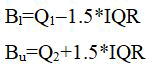
Here, a result lower than Bl and greater than Bu is considered as an outlier. Synthetic Minority Oversampling Technique (SMOTE) was also applied to balance the imbalanced data.
Feature selection
Data representation and intelligent diagnosis both depend on feature selection. One of the most popular feature selection methods is the elastic net. However, the features chosen rely on the training data and the regularized regression weights assigned to them are unrelated to their significance if used for feature ranking, which reduces the model's interpretability and extensibility.
According to Hastie, et al., the elastic net penalty aims to combine the gains of shrinkage and sparsity, which are both strengths of ridge regression and LASSO. By minimizing the elastic net estimator [19].
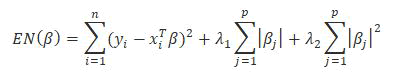
Due to the ridge regularization, the elastic net estimator can handle correlations between the predictors better than LASSO and due to the L1 regularization, sparsity is obtained. However, the bias issue present for LASSO is still present for elastic net.
However, the elastic net results in uneven Feature Selection (FS) [20]. The elastic net chooses new features and re-estimates their weights as the training set's data samples change.
Classification algorithms
This section discusses classification algorithms that are used to make predictions.
Logistic regression
Supervised machine learning techniques like logistic regression may be applied to both classification and regression issues. Probability is used in logistic regression to forecast how categorical data will be categorized. To forecast the result, input values can be blended linearly using a sigmoid or logistic function and coefficient values. The sigmoid function is used to estimate maximum likelihood using the most likely data and a probability between 0 and 1 is given to indicate whether or not an event will occur. When the decision threshold is applied, a categorization issue arises. There are several varieties of it, including binary (0 or 1), multinomial (three or more classes without any ordering) and ordinal (three or more classifications with ordering). It is an easy model to use and can provide accurate predictions. The following logistic regression equation determines the likelihood that input X should be classified in class 1:
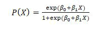
Here β0 is bias and β1 is the weight that is multiplied by input X.
K-nearest neighbour
The supervised machine learning method K-Nearest Neighbour (KNN) may be applied to classification and regression issues. In KNN, if a data point's target value is absent, the k closest data points are found in the training set and the average value of those points is supplied instead. The mode of k labels is assigned or returned in classification, while the mean of k labels is tuned in regression. It is a basic method that is used for categorization when prior knowledge of the data is lacking. The nearest data points can be determined using distance metrics like the manhattan distance or the Euclidean distance. Even with enormous amounts of noisy data, it can still yield superior findings and predictions.
Support Vector Machine (SVM)
In order to perform classification, a hyper plane is created, with samples from one class lying on one side and samples from another class lying on the other. The hyper plane is optimized to achieve the most excellent possible separation between two classes. The data points from classes that are closest to the hyper plane are considered to support vectors [21].
A hyper plane can be created using the equation shown below:
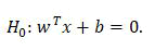
Two more hyper planes H1 and H2 are created in parallel to the constructed hyper-planes as given in the following equations:
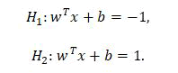
Hyper-planes should be satisfying the constraints given by following equations for each input vector Ij:
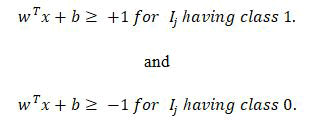
Hyper plane separating two classes in SVM.
Random Forest (RF)
Both classification and regression issues may be solved with random forest. It takes advantage of supervised machine learning. A random forest is an ensemble of decision trees that uses many trees for training and prediction. Every sample from the dataset is taken for repeated sampling and for each sample, a decision tree is created. The majority voting method is used to predict outcomes based on combining all decision trees. The functionality of RF is shown in Figure 3.

Figure 3: Random forest algorithm.
RF can be turned for increased accuracy by optimizing parameters such as the number of estimators, minimum size of node and number of features used for to split the node, etc. In this research, authors had done hyper parameter tuning of RF using grid search CV method [22-25].
Ada Boost (AB)
In order to create a more reliable classifier, the AdaBoost or adaptive boosting method combines a number of weak classifiers. Based on 1000 samples, this method generates the predicted accuracy. As illustrated in, occurrences from the training dataset are weighted.
Where xi is the ith training instance and N is the frequency of training occurrences. Each input variable receives an output from the decision tree. Equation 15 is then used to get the misclassification rate.
Boosting simply means combining several simple trainers to achieve a more accurate prediction. AdaBoost fixes the weights which may vary for both samples and classifiers. The final classification formula shown in equation.
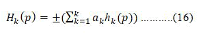
Equation (16), where k is the total number of weak classifiers hk (p), is a linear combination of all weak classifiers (simple learners). The working of AdaBoost algorithm is shown in Figure 4.

Figure 4: AdaBoost algorithm.
Artificial Neural Network (ANN)
Machine learning in neural networks includes artificial neural networks. The functioning of ANNs is compared to that of the human brain. It is built to mimic a human neuron cell in that it learns from data, classifies and anticipates output in the same manner as a cell receives input and responds. The statistical architecture used to find sophisticated problem solving is nonlinear. As illustrated an ANN structure comprises a data input layer, one or more hidden layers and an output layer with many nodes that resemble neurons in the human brain.
Nodes in an ANN function as the input of the input layer, taking information from the output world and feeding it to the hidden layer, like how neurons interact. After some data processing, the hidden layer finds the pattern. The concealed layer may have one or more layers. Multi-Layer Perceptron (MLP), which we shall explore in the next point, is an ANN with several hidden layers and back propagation. Once everything has been processed, it sends the categorized data to the output layer. An activation function is used to transform an input function into an output function; there are many distinct activation functions, including logistic, sigmoid, tanh and linear. Recently, ANNs have gained more popularity and are utilized in various industries, including medicine, image identification, speech recognition and facial recognition. However, employing the proper activation function and ANN parameters may provide significantly superior predictions (Figure 5).

Figure 5: The basic structure of ANN.
Multi Layer Perceptron (MLP)
When an ANN uses many hidden layers with back propagation instead of a single hidden layer, this is known as a multi-layer perceptron (more than three layers, including the input and output layer). A feed forward network is MLP (a cycle is not formed between connections). It operates by receiving input from other perceptrons, giving each node a weight and then sending that information to the hidden layer. The output layer is fed from concealed, as well. The anticipated value (derived during input processing or back propagation) and actual output are used to calculate the error value [30]. Back propagation between the hidden layer and output layer is done to minimize. The network does feed-forward after back propagation.
Classifier validation method: Validation of the prediction model is an essential step in machine learning processes. In this study, the K-Fold cross-validation method is applied to validating the results of the above mentioned classification models.
K-Fold Cross-Validation (CV): In K-Fold CV, the whole dataset is split into k equal parts. The (k-1) parts are utilized for training and the rest is used for the testing at each iteration. This process continues for k-iteration. Various researchers have used different values of k for CV. Here k=10 is used for experimental work because it produces good results. In tenfold CV, 90% of data is utilized for training the model and the remaining 10% of data is used for the testing of the model at each iteration.
Performance measure indices
The accuracy, sensitivity, specificity, f1-score, recall, Mathew Correlation-Coefficient (MCC) and AUC-score assessment matrices have all been applied to evaluate the effectiveness of the classification algorithms implemented in this work. These metrics are all computed using the confusion matrix shown in Table 2.
| Predicted (no disease) | Predicted (heart disease) | |
|---|---|---|
| Actual (no disease) | TN | FP |
| Actual (heart disease) | FN | TP |
Table 2: Confusion matrix.
The model predicts that the patient does not have cardiac disease, suggesting that the patient is healthy. True Negative (TN) in the confusion matrix shows that the patient does not have cardiac disease.
The model correctly classified a person with heart disease if True Positive (TP) confirms that the patient has heart disease and the model predicts the same result.
False Positive (FP) results show that the patient does not have cardiac disease despite the model's prediction that they do; in other words, the model misclassified the patient as healthy. Another name for this is a type-1 error.
False Negative (FN) results indicate that the patient has heart disease despite the model's prediction that they do not; in other words, the model misclassifies patients with heart disease. This is also called a type-2 error.
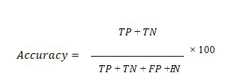
Accuracy: The following formula may be used to compute the accuracy of the classification model, which indicates the model's overall performance:
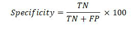
Specificity: A measure of specificity is the proportion of newly identified healthy persons to the total number of healthy people. It indicates that the prediction is negative and the person is healthy. The following is the specificity calculation formula
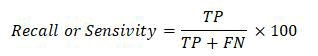
Sensitivity: Sensitivity is a ratio of the number of people with heart disease who are currently categorized as having the condition to the total number of people. It indicates that the model's prediction was accurate and that the person has heart disease. The following formula can be used to determine sensitivity:
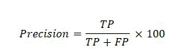
Precision: Precision is the difference between the actual and positive scores predicted by the classification model. To calculate precision, use the formula below.
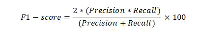
F1-score: F1-measure is the weighted measure of both recall and precision. Its value ranges between 0 and 1. If its value is one, it means the excellent performance of the classification algorithm and if its value is 0, it means the bad performance of the classification algorithm.
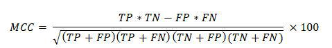
MCC: It is a correlation coefficient between the actual and predicted results. MCC gives resulting values between -1 and +1. Where -1 represents the completely wrong prediction of the classifier. 0 means that the classifier generates random prediction and +1 represents the ideal prediction of the classification models. The formula for calculating MCC values is given below:
The Area Under the Curve (AUC) and classification algorithm performance are closely associated, meaning that the greater the AUC value, the better the classification algorithm performance. The ROC of a classifier is described by the Area Under the Curve (AUC).
Results and Discussion
Patients' cardiac conditions were diagnosed using various classification methods, such as Logistic regression, K-nearest neighbor, support vector machine, random forest, Adaboost, artificial neural network and Multilayer perceptron. The UCI Cleveland dataset was implemented for the studies. Several medical factors from the dataset were used to diagnose heart disease. With class 1 denoting the presence of a disease and class 0 denoting the absence of a disease, these factors were utilized to accomplish classification. Seven instances in the dataset had missing values. These values were imputed using MICE algorithm. Application of this algorithm resulted in a complete dataset with no instance having missing value. System performance was measured on the scale of accuracy, sensitivity, specificity, precision, f1-measure, sensitivity, AUC-score and MCC. Results are validated using k-fold cross-validation method with k=10. In this method partitioning of the dataset is done into k groups. Performance of the model is evaluated using k-1 groups for the training of the model and one group for testing of the model. These steps of evaluating the model are repeated k times each time taking different training and testing groups.
Performance of classifiers with all features
At first, the experiments were performed on all features of the dataset without applying any kind of pre-processing or feature selection techniques. The performance of classifiers on the feature set is shown in Table 3. Classifier provided the highest performance on the full feature set, whereas SVM provided the lowest performance.
| Classification model | Accuracy | Sensitivity | Specificity | AUC | Precision | F1-score | MCC |
|---|---|---|---|---|---|---|---|
| LR | 0.81 | 0.88 | 0.75 | 0.9 | 0.77 | 0.82 | 0.63 |
| KNN (k=5) | 0.71 | 0.88 | 0.6 | 0.84 | 0.69 | 0.71 | 0.51 |
| SVM | 0.68 | 0.63 | 0.63 | 0.73 | 0.65 | 0.68 | 0.35 |
| RF | 0.99 | 0.98 | 1 | 1 | 1 | 0.99 | 0.98 |
| AB | 0.94 | 0.91 | 0.97 | 0.98 | 0.96 | 0.93 | 0.88 |
| ANN | 0.78 | 0.77 | 0.73 | 0.84 | 0.78 | 0.77 | 0.6 |
| MLP | 0.8 | 0.93 | 0.7 | 0.88 | 0.74 | 0.82 | 0.64 |
Table 3: Performance of classifiers on full feature set.
Performance improvement using class balancing
After applying the unbalanced classes, the performance of the classifiers has been further improved by maintaining the balance of the classes. SMOTE algorithm was applied for class balancing.
It resulted in 526 instance of both class 0 and class 1. Impact of class balancing on the performance of classifiers is shown in Table 4.
| Classification model | Accuracy | Sensitivity | Specificity | AUC | Precision | F1-score | MCC |
|---|---|---|---|---|---|---|---|
| LR | 0.83 | 0.89 | 0.76 | 0.91 | 0.79 | 0.84 | 0.66 |
| KNN (k=7) | 0.72 | 0.69 | 0.74 | 0.83 | 0.73 | 0.71 | 0.43 |
| SVM | 0.68 | 0.68 | 0.68 | 0.72 | 0.68 | 0.68 | 0.35 |
| RF | 1 | 1 | 0.99 | 1 | 0.99 | 1 | 0.99 |
| AB | 0.95 | 0.94 | 0.96 | 0.97 | 0.96 | 0.95 | 0.91 |
| ANN | 0.84 | 0.84 | 0.84 | 0.81 | 0.84 | 0.84 | 0.68 |
| MLP | 0.81 | 0.91 | 0.7 | 0.9 | 0.75 | 0.83 | 0.63 |
Table 4: Performance improvement using class balancing.
An increase, decrease and unchanged of accuracy, sensitivity, specificity, AUC, precision, f1-measure and MCC of classifiers with and without class balancing shown in Figures 6-12 respectively.

Figure 6: Accuracy of classi ier using class balancing.

Figure 7: Sensitivity of classifier using class balancing.

Figure 8: Specificity of classifiers after class balancing.

Figure 9: AUC score of classifiers after class balancing.

Figure 10: Precision of classifiers after class balancing.

Figure 11: F1-measure of classifiers after class balancing.

Figure 12: MCC of classifiers after class balancing.
According to Table 5, the performance score of the ANN and LR models increased after class balancing. On the other hand, SVM and MLP model scores remain almost same, while the model performance score reduced of RF.
| Performance classifiers | Increased | Decreased | Unchanged |
|---|---|---|---|
| Accuracy | LR, KNN, ANN | RF, AB | SVM, MLP |
| Sensitivity | LR, ANN, MLP | AB | KNN, SVM, RF |
| Specificity | KNN, ANN | RF | LR, SVM, MLP |
| AUC score | --- | LR, KNN, SVM, RF | AB, ANN, MLP |
| Precision | LR, KNN, ANN, MLP | ---- | SVM, RF, AB |
| F-measure | LR, ANN, AB | --- | KNN, SVM, RF, MLP |
| MCC | LR, AB, ANN | KNN | SVM, RF, MLP |
Table 5: Performance of all classifiers with and without balancing.
Performance improvement using feature selection
The elastic net feature selection approach is used to identify the optimum feature set that decreases computing cost and improves classifier performance (Table 6). The best results are still noted on the subset of (n=7) to pick the ideal feature space that reduces computing cost and enhances the classifiers' performance. Table 7 shows the projected outcomes of the best chosen feature space using a 10-fold CV and the optimal value of lambda used 0.03 because this value of Root Mean Sum of Squares (RMSE) is low. The classifiers’ performance on optimal feature space of elastic net feature selection algorithm at reported in Table 8.
| Lamda | RMSE |
|---|---|
| 0 | 0.355985 |
| 0.001 | 0.355956 |
| 0.002 | 0.355951 |
| 0.003 | 0.35597 |
| 0.004 | 0.356012 |
| 0.005 | 0.356077 |
Table 6: Optimum value of lambda for elastic net regression.
| SL no. | Features | Feature code | Score |
|---|---|---|---|
| 1 | 2 | SEX | 0.178 |
| 2 | 8 | THAL | 0.117 |
| 3 | 12 | EIA | 0.112 |
| 4 | 3 | CPT | 0.104 |
| 5 | 9 | VCA | 0.09 |
| 6 | 7 | RECG | 0.068 |
| 7 | 10 | PES | 0.05 |
Table 7: Selected features by elastic net algorithm and their scores
| Classification model | Accuracy | Sensitivity | Specificity | AUC | Precision | f1-score | MCC |
|---|---|---|---|---|---|---|---|
| LR | 0.82 | 0.85 | 0.78 | 0.9 | 0.83 | 0.84 | 0.66 |
| KNN (k=7) | 0.87 | 0.9 | 0.84 | 0.95 | 0.87 | 0.89 | 0.74 |
| SVM | 0.88 | 0.92 | 0.83 | 0.95 | 0.87 | 0.9 | 0.76 |
| RF | 0.92 | 0.94 | 0.91 | 0.98 | 0.92 | 0.93 | 0.84 |
| AB | 0.83 | 0.85 | 0.81 | 0.92 | 0.85 | 0.85 | 0.66 |
| ANN | 0.88 | 0.86 | 0.8 | 0.92 | 0.84 | 0.85 | 0.67 |
| MLP | 0.86 | 0.88 | 0.83 | 0.94 | 0.87 | 0.87 | 0.71 |
Table 8: Performance using elastic net feature selection algorithm.
Feature selection improved the performance of all classifiers except RF and Adaboost. LR, KNN, ANN and MLP accuracy increased by only 1%, 16%, 10% and 6%. A maximum increase of 20% was observed in the accuracy of SVM and a maximum decrease of 11% was observed in Adaboost. The best results were achieved in SVM. Sensitivity, specificity, AUC, precision, f1- measure and MCC of SVM increased by only 29%, 20%, 22%, 22% and 41%. After feature selection, performance scores decrease in Adaboost classifier. An improvement performance of all classifiers with feature selection is shown in Figures 13-19.

Figure 13: Accuracy scores of classifiers using feature selection.

Figure 14: Sensitivity of classifiers after feature selection.

Figure 15: Specificity of classifiers using feature selection.

Figure 16: Increase in AUC score of classifiers using feature selection.

Figure 17: Increase in precision of classifiers using feature selection.

Figure 18: Increase in F-measure of classifiers using feature selection.

Figure 19: Increase in the MCC score of classifiers using feature selection.
Results indicates that random forest provided the highest performance in combination with MICE, elastic net and SMOTE. Dimensionality reduction using Feature selection the performance of RF slightly decreasing compared to without feature selection and class balancing. KNN, SVM and ANN performance increased gradually after dimensionality reduction.
Conclusion
Heart disease is one of the most devastating and fatal chronic disease that rapidly increase in both economically developed and undeveloped countries and cause death. This damage can be reduced considerably if the patient is diagnosed in the early stages and proper treatment is provided to his/her. The major cause of loss of life in heart disease is a delay in its detection. To assess the performance of classification algorithms various performance evaluation metrics were used such as accuracy, sensitivity, specificity, AUC, precision, f1-measure and MCC. In this paper we showed that the comparison the performance scores of LR, KNN, SVM, RF, AB and MLP classifiers with and without feature selection and class balancing. We observed that the performance increased ANN and LR after class balance and remain constant in SVM and MLP. The classification accuracies of the top two classification algorithms, i.e., RF and Adaboost, on full features were 99% and 94%, respectively. After applying feature selection algorithms, the classification accuracy of RF with elastic net feature selection algorithm slightly decreases from 99% to 92%. The accuracy of Adaboost decreases from 94% to 83%. However, the performance of classifiers was increased after class balance and feature selection, such as KNN, SVM and MLP. After class balancing and feature selection, the SVM classifier provides the best performance. In the future, the researchers plan to investigate with other feature selection approaches, such as Ant Colony optimization and particle swarm optimization, in order to further enhance the performance system. The authors also intend to use deep learning methods to create a system for diagnosing heart disease.
References
- Ayon SI, Islam MM, Hossain MR (2022) Coronary artery heart disease prediction: a comparative study of computational intelligence techniques. IETE J Res 68:2488-2507
[Crossref] [Googlescholar] [Indexed]
- Patil SB, Kumaraswamy Y (2009) Intelligent and effective heart attack prediction system using data mining and artificial neural network. Eur J Sci Res 31:642-656
- Vanisree K, Singaraju J (2015) Decision support system for congenital heart disease diagnosis based on signs and symptoms using neural networks. Int J Comput Appl 19:6-12
- Edmonds (2005) In Proceedings of AISB Symposium on Socially Inspired Computing. 1â??12
- Methaila A, Kansal P, Arya H, Kumar P (2014) Early heart disease prediction using data mining techniques. Sci Inf Technol J 28:53-59
- Ponikowski P, Anker SD, AlHabib KF, Cowie MR, Force TL, et al. (2014) Heart failure: Preventing disease and death worldwide. ESC Heart Fail 1:4-25
- Gandhi M, Singh SN (2015) Predictions in heart disease using techniques of data mining. IEEE 520-525
- Bashir S, Qamar U, Khan FH, javed MY (2014) MV5: A clinical decision support framework for heart disease prediction using majority vote based classifier ensemble. Arab J Sci Eng 39:7771-7783
- Olaniyi EO, Oyedotun OK, Adnan K (2015) Heart diseases diagnosis using neural networks arbitration. Int J Intell Syst Appl 7:75-82
[Crossref] [Googlescholar] [Indexed]
- Thomas J, Princy RT (2016) Human heart disease prediction system using data mining techniques. 2016 International Conference on Circuit, Power and Computing Technologies (ICCPCT).
[Crossref] [Googlescholar] [Indexed]
- Verma L, Srivastava S, Negi PC (2016) A hybrid data mining model to predict coronary artery disease cases using non-invasive clinical data. J Med Syst 40:17
[Crossref] [Googlescholar] [Indexed]
- Verma L, Srivastava S (2016) A data mining model for coronary artery disease detection using noninvasive clinical parameters. Indian J Sci Technol 9:1-6
[Crossref] [Googlescholar] [Indexed]
- Pahwa K, Kumar R (2017) "Prediction of heart disease using hybrid technique for selecting features," 2017 4th IEEE Uttar Pradesh Section International Conference on Electrical, Computer and Electronics (UPCON), Mathura. 500â??504
- Xu S, Zhang Z, Wang D, Hu J, Duan X, et al. (2017) Cardiovascular risk prediction method based on CFS subset evaluation and random forest classification framework. In 2017 IEEE 2nd International Conference on Big Data Analysis (ICBDA) 228-232
- Jabbar MA, Deekshatulu BL, Chandra P (2016) Prediction of heart disease using random forest and feature subset selection. In: Innovations in bio-inspired computing and applications. Springer 187-196
- Latha CBC, Jeeva SC (2019) Improving the accuracy of prediction of heart disease risk based on ensemble classification techniques. Inf Med Unlocked 16:100203
- Terrada O, Hamida S, Cherradi B, Raihani A, Bouattane O (2020) Supervised machine learning based medical diagnosis support system for prediction of patients with heart disease. Adv Sci Technol Eng Syst J 5:269-277
[Crossref] [Googlescholar] [Indexed]
- Tama BA, Im S, Lee S (2020) Improving an intelligent detection system for coronary heart disease using a two-tier classifier ensemble. Biomed Res Int 2020:1-10
- Saez JA, Krawczyk B, Wozniak M (2016) Analyzing the oversampling of different classes and types of examples in multi-class imbalanced datasets. Pattern Recogn 57:164-178
[Crossref] [Googlescholar] [Indexed]
- Azur MJ, Stuart EA, Frangakis C, Leaf PJ (2011) Multiple imputation by chained equations: what is it and how does it work. Int J Methods Psychiatr Res 20:40-49
[Crossref] [Googlescholar] [Indexed]
- Rahman MR, Islam T, Zaman T, Shahjaman M, Karim MR, et al. (2019) Identification of molecular signatures and pathways to identify novel therapeutic targets in Alzheimerâ??s disease: Insights from a systems biomedicine perspective. Genomics 112:1290-1299
[Crossref] [Googlescholar] [Indexed]
- Shahriare Satu M, Atik, ST, Moni MA (2020) A novel hybrid machine learning model to predict diabetes mellitus. Springer 453-465
- Zou H, Hastie T (2005) Regularization and variable selection via the elastic net. J R Statist Soc 67:301-320
[Crossref] [Googlescholar] [Indexed]
- Rani P, Kumar R, Jain A, Lamba R (2020) Taxonomy of machine learning algorithms and its applications. J Comput Theror Nanosci 17:2509-2514
[Crossref] [Googlescholar] [Indexed]
- Dangare C, Apte S (2012) A data mining approach for prediction of heart disease using neural networks. Int J Eng Technol 3:11


Open Access Journals
- Aquaculture & Veterinary Science
- Chemistry & Chemical Sciences
- Clinical Sciences
- Engineering
- General Science
- Genetics & Molecular Biology
- Health Care & Nursing
- Immunology & Microbiology
- Materials Science
- Mathematics & Physics
- Medical Sciences
- Neurology & Psychiatry
- Oncology & Cancer Science
- Pharmaceutical Sciences