Multi-Scale Regional Groundwater Model Development and Calibration
Mingjie Chen*, Osman A Abdalla and Azizallah Izady
Water Research Center, Sultan Qaboos University, Muscat, Oman
- *Corresponding Author:
- Mingjie Chen
Senior Hydrogeologist
Water Research Center, Sultan Qaboos University
Al Khoudh, Muscat 123, Oman
Tel: 968-24143202
E-mail: cmj1014@yahoo.com
Received Date: April 04, 2018; Accepted Date: April 24, 2018; Published Date: May 04, 2018
Citation: Chen M, Abdalla OA, Izady A (2018) Multi-Scale Regional Groundwater Model Development and Calibration. J Water Pollut Control. Vol.1 No.2:4
Abstract
As an important groundwater resources management tool, groundwater flow model has been extensively used for estimating water balance and flow dynamics of aquifers. In addition, regional-scale flow model with coarse grid can provide hydrologic context to establish boundary conditions of the site-scale contaminant transport model with fine grid. In this study, a regional groundwater flow model is developed for a hydrogeological drainage basin, and calibrated using water level measurements. Particle tracking is then conducted to estimate the travel path of contaminants from the potential sources, which helps to define the domain for transport sub-model. Parent-child grid coupling between coarse flow model and higher-resolution transport model are demonstrated using finite element control volume techniques.
Keywords
Multi-scale; Groundwater model; Control volume finite element; Grid coupling
Introduction
During basin-scale hydrologic modeling, grid coupling is useful when fine grids are required to minimize numerical dispersion in embedded contaminant transport calculation. In some situation, a high-resolution sub-model is required to incorporate into a developed large-scale coarse model to simulate a newly discovered contaminant source. Finite difference (FD), finite element (FEM), and control volume finite element (CVFE) numerical discretization techniques have been used in coupling models. Traditional FD methods require head and flux interpolation with model iteration to minimize the errors caused by abrupt grid size change from a coarse parent grid to a fine child grid [1,2]. On the contrary, FEM and CVFE can handle the transition from the course to fine grids without iteration owing to its inherently flexible grids. While FEM methods have been widely understood, only a few descriptions on CVFE in model coupling are reported in literature [3-5]. In this study, both a coarse-grid and an associated hybrid coarsefine grid basin model are developed and discussed using CVFE techniques. Grid coupling using CVFE is introduced in Section 2. Next in Section 3 and 4, a basin-scale hydrologic model with CVFE grids is developed using FEHM (finite element heat and mass transfer) code [6] and calibrated by parameter estimation software PEST [7]. Particle tracking is also conducted to assess potential contaminant travel paths. In Section 5, comparison analysis is conducted between results simulated by hybrid model with coarse-fine grid and those by uniform-grid model. The study is summarized and concluded in Section 6.
Materials and Methods
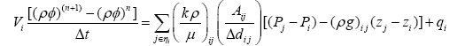
The CVFE method can be described as a block-centered finite difference method on irregularly shaped control volumes. Nonorthogonal connections are allowed so long as they have positive areas. The rules for node spacing and geometry were developed by voronoi, [8]. The voronoi volume is formed by boundaries that are orthogonal to the lines joining adjacent nodes and that intersect the midpoints of the lines [9]. The material balance equations that describe the flow of water discretized via CVFE method may be written for every grid block as:
 (1)
(1)
where, is the set of neighbor nodes of  is the Voronoi volume associate with node
 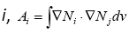 is the area between connected nodes i and j, and dij is the distance between nodes i and j. Ni is the usual finite element polynomial basis function, and we have Ni =1 at node i, Ni =0 at all other nodes. k is the permeability, ρ is the water density, and μ is the water viscosity. n and n+1 indicate the successive time step. qi is the flow source or sink term (Figure 1).

Figure 1: Illustration of the nodes and connectivity in transition zone (1:2 ratio) for (a) finite difference; (b) control volume finite element.
Figure 1b shows the CVFE equivalent to FD in Figure 1a. Obviously, the inherent fixed connectivity of FD requires additional treatment to insure mathematical consistency in resolution transient zone [1]. In contrast, CVFE can easily address the transition between high and low-resolution regions with all connections. It should be noted that when CVFE methods are applied to orthogonal finite difference grids they exactly reproduce finite difference equations in regions other than transition zone. The resolution ratio between parent and child grid can be increased as needed as shown in Figure 2.

Figure 2: Transition zone between high and low resolution (1:4 ration) for CVFE grid.
Flow model development
The numerical basin model was constructed using the FEHM code [6], which is capable of simulating mass and heat transfer in both confined and unconfined aquifers. For this study, the isothermal confined and unconfined aquifer module was used. The model domain within the drainage boundary is shown in Figure 3. The basin rock was delineated into six stratigraphic units which were implemented in the numerical model by digitizing implied stratigraphic boundaries from a USGS report. The basin topography is derived from DEM data. The model domain is about 55 km by 55 km horizontally, and the vertical elevation is from 1200 m to 3000 m. Based on the geological model, the basin model is discretized into a CVFE grid system consisting of 700,000 nodes of which about 400,000 are active. As shown in Figure 4, the horizontal grid resolution is uniform 500 m by 500 m, and the vertical node space is variable from 20 m to 50 m (Figure 3 and Figure 4).

Figure 3: The basin drainage and simplified stratigraphy.

Figure 4: Numerical grid blocks for the 3D basin model. (a) bird view; (b) cross section.
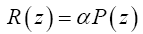
The two creek drainages in the basin were delineated and digitalized into 25 creeks and gulches (Figure 5). These creeks are simulated as constant head boundaries in the numerical model. The recharge applied to the surface layer was estimated by a simple function of elevation z [10]:
 (2)
(2)
Where P(z) is the amount of annual precipitation falling at elevation z, and α is the fraction of that precipitation recharging the basin aquifers. Aquifer recharge occurs primarily at high elevations (>7000 ft or 2134 m). In the target region, α is less than 0.3 at high elevations where most recharge occurs, and α is zero at low elevations where evapotranspiration exceeds precipitation. Annual precipitation ranges from about 300 to 510 mm between altitudes of 1,680 m and 2,440 m. Using this information, we extrapolate a linear relationship P(z) = 300+(z- 1680)*0.28, resulting in the recharge map shown in Figure 5. The map also shows discharge along the creeks. All discharge occurs to the two creeks and their tributaries only. No inflow or outflow is allowed on the model boundary which is also the drainage boundary (Figure 5).

Figure 5: Recharge map input to the basin model. Positive values indicate discharge along the creeks, and negative values represent recharge zone whose elevation is above 7000 feet (2134 m).
Flow model calibration (Table 1 and Figure 6)
Table 1. Estimated permeability of stratigraphic units represented in the model
| Layer | Color in Figure 3a | Horizontal Permeability (m2) | Vertical Permeability (m2) | ||
|---|---|---|---|---|---|
| Initial | Calibratedb | Initial | Calibratedb | ||
| 1 | Dark blue (bedrock) | 1.00E-18 | Fixed | 1.00E-18 | Fixed |
| 2 | Orange | 3.00E-13 | 2.30E-13 | 6.00E-15 | 5.18E-15 |
| 3 | Yellow | 3.00E-13 | 2.60E-13 | 6.00E-15 | 5.47E-15 |
| 4 | Red orange | 6.00E-14 | 4.60E-14 | 6.00E-16 | 5.82E-16 |
| 5 | Dark green | 3.60E-13 | 3.20E-13 | 1.80E-13 | 1.74E-13 |
| 6 | Light green | 7.20E-14 | 7.50E-14 | 3.60E-14 | 4.00E-14 |
aLayers are indexed from bottom to top at Figure 3.
bEstimated by traditional calibration.

Head measurements from 98 wells are used to calibrate the 3D basin model (Figure 6). The horizontal and vertical permeability of the 5 layers (excluding the layer 1 bedrock) are considered homogeneous and chosen as the estimated targets. As shown in Table 1, the initial permeability values are chosen according to the USGS report and the calibration are performed using PEST code. As shown in Figure 7a, simulated heads don’t match the measurements very well, especially at locations of high elevations. The large discrepancy between the simulated and measured heads might be due to the assumption of uniform permeability for each layer (Figure 7).

Figure 7: Scatter plot of measured and simulated heads at 98 wells by (a) traditional calibration, and (b) pilot point’s calibration.
To address this challenge, pilot point’s method in PEST software is applied for the basin model calibration. Instead of uniform values on each layer, pilot points calibration estimate permeability in pilot points at specified locations of each layer. The number of pilot points is 22, 11, 23, 17, and 48 at layer 2, 3, 4, 5, and 6, totaling 121 for the calibration. It should be noted that the number of parameters to be estimated is the number of pilot points. Inverse modeling with so many parameters may cause illposed issue. Truncated singular value decomposition technique is used to reduce the parameter space dimension. By assuming the permeability parameter as a random field, the values of permeability at every node of the layer are interpolated using those values at pilot points by geo-statistical techniques (e.g., krigging). Figure 8a presents the heterogeneous permeability of the top layer (layer 6) estimated by pilot points calibration. The heterogeneous permeability field of each layer is input to the basin model to simulate the flow dynamics and the resulted heads on the top layer are shown in Figure 8b. It is seen that overall trend is that heads decrease from the peripheral mountain area to the central north drainage zone, generally in line with the topography and applied recharge. The simulated heads at observation wells are compared to the measurements, and the close match demonstrates considerable improvement by using the pilot point calibration over the traditional calibration approach (Figure 7b, Figure 8).

Figure 8: Contour map of (a) Log-transformed permeability and (b) head of the top layer of the basin model calibrated by pilot points method.
To facilitate development of transport model, potential flow
paths for the contaminant should be evaluated. Particle tracking methods are implemented to simulate the moving tracks of synthetic contaminants released from the targeted sources with the simulated flow field by the basin model. The simulated path lines indicate the pollutants from the sources will be discharged to the two creeks north of the site (Figure 9a). The average travel time the layer 3, 4, and 5 are 690, 538, and 280 years, respectively (Figure 9b). The particles from the lower layers move slower because they have to cross the low permeable layer 4 northward and upward. The particle tracking also suggests that the transport model domain (Figures 6 and 10) is appropriately defined and covers the entire potential contaminant transport area (Figure 9).

Figure 9: Flow pathlines of the particles released from the potential contaminated site: (a) plan view and (b) vertical slice viewed from the east.
Hybrid model
Owing to the flexibility of CVFE grids discussed above, a hybrid Basin model was conveniently developed with fine resolution around the contaminated site based on the uniform-grid model (Figure 9). The grid resolution smoothly transitions from 500m (plan view grid block size) away from the contaminated site to 62.5 m near the site (1:8 ratio). The fine resolution extends to the fluid discharge areas along the creeks, covering potential contaminant moving area estimated by particle-tracking simulation. The first task is to insure consistency between this hybrid model and the calibrated uniform-grid model. Using the permeability values from the calibrated model, the hybrid model was evaluated with field measurements. The average relative error of heads at 98 observations is only 0.07%, and that of the discharge is less than 5%. The comparison suggests close match of the head and discharge between the hybrid model and the uniform grid model. This result also demonstrates that the grid resolution is appropriate for the coarse grid model (Figure 10).

Figure 10: Hybrid basin model with high-resolution grid near contaminant site (1:8 ratio). The square denotes the potential contaminated site.
Conclusion
This study presents a general procedure for development and calibration of a regional groundwater flow model. The powerful capability of CVFE to couple multi-scale sub-models into the coarse large-scale model is also demonstrated. The basin flow model provides necessary boundary conditions for the contaminant transport model. The future work is to develop the separate transport model. The domain is approximately 5 km by 7 km, covering potential contaminant moving area according particle tracking simulation (Figure 10). The mesh system consists of 500,000 grid blocks with 62.5 m space. The fixed head boundary is obtained from the coarse-grid basin model in this study. Unlike predefined hybrid grid, the refined child grids could be embedded anywhere, anytime during the large-scale basin model development. This posterior patch capability will provide a promising foreground of applications in multi-scale saturatedunsaturated flow system and subsurface-surface watershed modeling area (Figure 11).

Figure 11: The domain and grid of the transport model.
Acknowledgement
This work was supported by Sultan Qaboos University internal grant #IG/DVC/WRC/17/01 and BP Oman grant #BP/DVC/ WRC/18/01. We would like to thank the Center for Information System and Water Research Center at Sultan Qaboos University for computing facility management.
References
- Mehl S, Hill MC (2002) Development and evaluation of a local grid refinement method for blockcentered finite-difference ground-water models using shared nodes. Adv Water Resour 25: 497-511.
- Mehl S, Hill MC (2004) Three-dimensional local grid refinement for block-centered finite-difference groundwater models using iteratively coupled shared nodes: a new method of interpolation and analysis of errors. Adv Water Resour 27: 899-912.
- Forsyth P (1990) A control volume finite element method for local mesh refinement, Paper SPE 18425, presented at the SPE Symposium on Reservoir Simulation, Houston, TX.pp: 267-278.
- Keating EH, Vesselinov VV, Kwicklis E, Lu Z (2003) Coupling basin- and site-scale inverse models of the Espanola aquifer. Ground Water 41: 200-211.
- Zyvoloski GA, Vesselinov VV (2006) An investigation of numerical grid effects in parameter estimation. Ground water 44: 814-825.
- Zyvoloski GA, Robinson BA, Dash ZV, Trease LL (1997) Summary of the models and methods for the FEHM application: A finite element heat- and mass-transfer code. Los Alamos National Laboratory Report.
- Doherty J (2002) PEST: Model independent parameter estimation. Watermark Numerical Computing, Brisbane, Australia.
- Aurenhammer F (1991) Voronoi diagrams-A survey of fundamental geometric data structure. ACM ComputSurv 23: 345-405.
- Verma AK, Eswaran V (1996) Overlapping control volume approach for convection–diffusion problems. Int J Numer Methods Fluids 23: 865-882.
- Maxey GB, Eakin TE (1949) Ground water in White River Valley, White Pine, Nye, and Lincoln Counties, Nevada. Water Resources Bulletin No-8. Nevada State Engineer, United States, pp. 59.

Open Access Journals
- Aquaculture & Veterinary Science
- Chemistry & Chemical Sciences
- Clinical Sciences
- Engineering
- General Science
- Genetics & Molecular Biology
- Health Care & Nursing
- Immunology & Microbiology
- Materials Science
- Mathematics & Physics
- Medical Sciences
- Neurology & Psychiatry
- Oncology & Cancer Science
- Pharmaceutical Sciences