ISSN : 2349-3917
American Journal of Computer Science and Information Technology
Analysis of Molecular Variance (AMOVA): A Bio Mathematical Approach in Complete Genomes of SARS-CoV-2
Robson Da Silva Ramos*, Pierre Teodosio Felix, Dallynne Barbara Ramos Venancio and Eduarda Doralice Alves Braz Da Silva
Laboratory of Population Genetics and Computational Evolutionary Biology, UNIVISA, Vitória de Santo Antao, Pernambuco, Brazil
- *Corresponding Author:
- Robson Da Silva Ramos
Laboratory of Population Genetics and Computational Evolutionary Biology,
UNIVISA, Vitória de Santo Antao,
Pernambuco, Brazil
E-mail: pierrefelix@univisa.edu.br
Received Date: November 12, 2020; Accepted Date: November 25, 2020; Published Date: December 02, 2020
Citation: Ramos RDS, Felix PT, Venancio DBR, Silva EDABD (2020) Analysis of Molecular Variance (AMOVA): A Bio Mathematical Approach in Complete Genomes of SARS-CoV-2. Am J Compt Sci InformTechnol Vol.8 No.4: 65.
Abstract
In this work, we evaluated the levels of genetic diversity in 38 complete genomes of SARS-CoV-2, publicly available on the National Center for Biotechnology Information (NCBI) platform and from six countries in South America (Brazil, Chile, Peru, Colombia, Uruguay and Venezuela with 16, 11, 1, 1, 1, 7 haplotypes, respectively), all with an extension of 29, 906 bp and phred values ≥ 40. These haplotypes were previously used for phylogenetic analyses, following the alignment protocols of the MEGA X software where all gaps and uncoserved sites were extracted for the construction of phylogenetic trees. The specific methodologies for Paired FST estimators, Molecular Variance (AMOVA), Genetic Distance, mismatch, demographic and spatial expansion analyses, molecular diversity and evolutionary divergence time analyses, were obtained using 20,000 random permutations.
Keywords
Bioinformatics; Protocols; Phylogeny; AMOVA; Genetic diversity; SARSCoV- 2; Coronavirus; Bio mathematical
Methodology
Databank
The 38 complete genome sequences of SARS-CoV-2 from South America (Brazil, Chile, Peru, Colombia, Uruguay and Venezuela with 16, 11, 1, 2, 1, 7 haplotypes, respectively) all with 29, 906 pb extension and Phred values ≥ 40 and which now make up our study popset, were recovered from GENBANK on August 21, 2020.
Phylogenetic analyses
Nucleotide sequences previously described were used for phylogenetic analyses. The sequences were aligned using the MEGA X program and the gaps were extracted for the construction of phylogenetic trees [1].
Genetic structuring analyses
Paired FST estimators, Molecular Variance (AMOVA), Genetic Distance, mismatch, demographic and spatial expansion analyses, molecular diversity and evolutionary divergence time were obtained with the software Arlequin v 3.5 using 1000 random permutations [2,3]. The FST and geographic distance matrices were not compared. All steps of this process are described below.
For genetic diversity
Among the routines of LaBECom, this test is used to measure the genetic diversity that is equivalent to the heterozygosity expected in the groups studied. We used for this the standard index of genetic diversity H, described, which can also be estimated by the method proposed by PONS and PETIT [4,5].
For Site Frequency Spectrum (SFS)
According to LaBECom protocols, we used this local frequency spectrum analytical test (SFS), from DNA sequence data that allows us to estimate the demographic parameters of the frequency spectrum. Simulations are made using fastsimcoal2 software, available [6].
For molecular diversity indices
Molecular diversity indices are obtained by means of the average number of paired differences, as described by Tajima in 1993, in this test we used sequences that do not fit the model of neutral theory that establishes the existence of a balance between mutation and genetic drift [7,8].
For calculating theta estimators
Theta population parameters are used in our Laboratory when we want to qualify the genetic diversity of the populations studied. These estimates, classified as Theta Hom which aim to estimate the expected homozygosity in a population in equilibrium between drift and mutation and the estimates theta (S), theta (K) and theta (π) [8-10].
For the calculation of the distribution of mismatch
In LaBECom, analyses of the mismatch distribution are always performed relating the observed number of differences between haplotype pairs, trying to define or establish a pattern of population demographic behavior [11-13].
For pure demographic expansion
This model is always used when we intend to estimate the probability of differences observed between two haplotypes not recombined and randomly chosen, this methodology in our laboratory is used when we assume that the expansion, in a haploid population, reached a momentary balance even having passed through generations, of sizes 0N to 1N. In this case, the probability of observing the S differences between two nonrecombined and randomly chosen haplotypes is given by the probability of observing two haplotypes with S differences in this population [14].
For spatial expansion
The use of this model in LaBECom is usually indicated if the reach of a population is initially restricted to a very small area, and when one notices signs of a growth of the same, in the same space and over a relatively short time. The resulting population generally becomes subdivided in the sense that individuals tend to mate with geographically close individuals rather than random individuals [15]. To follow the dimensions of spatial expansion, we at LaBECom always take into account:
L: Number of loci
Gamma Correction: This fix is always used when mutation rates do not seem uniform for all sites.
nd: Number of substitutions observed between two DNA sequences.
ns: Number of transitions observed between two DNA sequences.
nv: Number of trans versions observed between two DNA sequences.
ω: G+C ratio, calculated in all DNA sequences of a given sample.
Paired difference: Shows the number of loci for two haplotypes different.
Percentage difference: This difference is responsible for producing the percentage of loci for which two haplotypes are different.
For haplotype inferences
We use these inferences for haplotype or genotypic data with unknown gametic phase. Following our protocol, inferences are estimated by observing the relationship between haplotype i and xi times its number of copies, generating an estimated frequency (^pi) [16]. With genotypic data with unknown gametic phase, the frequencies of haplotypes are estimated by the maximum likelihood method, and can also be estimated using the expected Maximization (MS) algorithm.
For the method of jukes and cantor
This method, when used in LaBECom, allows estimating a corrected percentage of how different two haplotypes are. This correction allows us to assume that there have been several substitutions per site, since the most recent ancestor of the two haplotypes studied. Here, we also assume a correction for identical replacement rates for all four nucleotides A, C, G and T.
For kimura method with two parameters
Much like the previous test, this fix allows for multiple site substitutions, but takes into account different replacement rates between transitions and trans versions.
Tamura method
We at LaBECom understand this method as an extension of the 2-parameter Kimura method, which also allows the estimation of frequencies for different haplotypes. However, transition-trans version relationships as well as general nucleotide frequencies are calculated from the original data.
Tajima and NEI method
At this stage, we were also able to produce a corrected percentage of nucleotides for which two haplotypes are different, but this correction is an extension of the Jukes and Cantor method, with the difference of being able to do this from the original data.
Tamura and nei model
As in kimura's models 2 parameters a distance of Tajima and Nei, this correction allows, inferring different rates of transversions and transitions, besides being able to distinguish transition rates between purines and pyrimidines.
For estimating distances between haplotypes produced by RFLP
We use this method in our laboratory when we need to verify the number of paired differences scouting the number of different alleles between two haplotypes generated by RFLP.
To estimate distances between haplotypes produced microsatellites
P In this case, what applies is a simple count of the number of different alleles between two haplotypes. Using the sum of the square of the differences are repeated sites between two haplotypes [17].
Minimum spanning network
To calculate the distance between OTU (Operational Taxonomic Units) from the paired distance matrix of haplotypes, we used a Minimum Spanning Network (MSN) tree, with a slight modification of the algorithm described. We usually use free software written in Pascal called MINSPNET. EXE running to DOS language previously available [18].
For genotypic data with unknown gametic phase
EM algorithm: To estimate haplotypic frequencies we used the maximum likelihood model with an algorithm that maximizes the expected values. The use of this algorithm in LaBECom, allows to obtain the maximum likelihood estimates from multilocal data of gamtic phase is unknown (phenotypic data). It is a slightly more complex procedure since it does not allow us to do a simple gene count, since individuals in a population can be heterozygous to more than one locus.
ELB algorithm: Very similar to the previous algorithm, ELB attempts to reconstruct the gametic phase (unknown) of multilocal genotypes by adjusting the sizes and locations of neighboring loci to explore some rare recombination.
For neutrality tests
Ewens-Watterson homozygosis test: We use this test in LaBECom for both haploid and diploid data. This test is used only as a way to summarize the distribution of allelic frequency, without taking into account its biological significance. This test is based on the sampling theory of neutral [19,20]. It is now limited to sample sizes of 2,000 genes or less and 1,000 different alleles (haplotypes) or less. It is still used to test the hypothesis of selective neutrality and population balance against natural selection or the presence of some advantageous alleles.
Ewens-Watterson-Slatkin test: It is used in our protocols when we want to compare the probabilities of random samples with those of observed samples [21].
Chakraborty's test of population amalgamation: This test serves to calculate the observed probability of a randomly neutral sample with a number of alleles equal to or greater than that observed, it is based on the infinite allele model and sampling theory for neutral alleles [22].
Tajima selective neutrality test: We use this test in our Laboratory when DNA sequences or haplotypes produced by RFLP are short. It is using the model of infinite sites without recombination. It commutes two estimators using the theta mutation as a parameter [23].
FS FU test of selective neutrality: Also based on the model of infinite sites without recombination, the FU test is suitable for short DNA sequences or haplotypes produced by RFLP. However, in this case, it assesses the observed probability of a randomly neutral sample with a number of alleles equal to or less than the observed value. In this case the estimator used is θ.
For methods that measure inter population diversity
Genetic structure of the population inferred by molecular variance analysis (AMOVA): This stage is the most used in the LaBECom protocols because it allows knowing the genetic structure of populations measuring their variances, is essentially similar to other approaches based on analyses of gene frequency variance, but takes into account the number of mutations between haplotypes [24]. When the population group is defined, we can define a particular genetic structure that will be tested, that is, we can create a hierarchical analysis of variance by dividing the total variance into covariance components by being able to measure intra-individual differences, inter individual differences and/or inter population allocated differences.
Minimum Spanning Network (MSN) among haplotypes: In LaBECom, this tree is generated using the operational taxonomic units (OTU). This tree is calculated from the matrix of paired distances using a modification of the algorithm described.
Locus-by-locus AMOVA: We performed this analysis for each locus separately as it is performed at the haplotypic level and the variance components and f statistics are estimated for each locus separately generating in a more global panorama.
Paired genetic distances between populations: This is the most present analysis in the work of LaBECom. These generate paired FST parameters that are always used, extremely reliably, to estimate the short-term genetic distances between the populations studied, in this model a slight algorithmic adaptation is applied to linearize the genetic distance with the time of population divergence [25].
Reynolds Distance: Here we measured how much pairs of fixed N-size haplotypes diverged over T generations, based on FST indices.
Slatkin's linearized FST's: We used this test in LaBECom when we want to know how much two Haploid populations of N size diverged t generations behind a population of identical size and managed to remain isolated and without migration. This is a demographic model and applies very well to the phylogeography work of our laboratory [26].
Nei's average number of differences between populations: In this test we assumed that the relationship between the gross (D) and liquid (AD) number of Nei differences between populations is the increase in genetic distance between populations [27].
Relative population sizes: divergence between populations of unequal sizes: We used this method in LaBECom when we want to estimate the time of divergence between populations of equal sizes, assuming that two populations diverged from an ancestral population of N0 size a few t generations in the past, and that they have remained isolated from each other ever since. In this method we assume that even though the sizes of the two child populations are different, the sum of them will always correspond to the size of the ancestral population [28]. The procedure is based on the comparison of intra and inters populational (π's) diversities that have a large variance, which means that for short divergence times, the average diversity found within the population may be higher than that observed among populations. These calculations should therefore be made if the assumptions of a pure fission model are met and if the divergence time is relatively old. The results of this simulation show that this procedure leads to better results than other methods that do not take into account unequal population sizes, especially when the relative sizes of the daughter populations are in fact unequal.
Accurate population differentiation tests: We at LaBECom understand that this test is an analog of fisher's exact test in a 2 × 2 contingency table extended to a rxk contingency table. It has been described and tests the hypothesis of a random distribution of k different haplotypes or genotypes among r populations [29].
Assignment of individual genotypes to populations: Inspired by what had been described in this method determines the origin of specific individuals, knowing a list of potential source populations and uses the allelic frequencies estimated in each sample from their original constitution [30-32].
Detection of loci under selection from F-statistics: We use this test when we suspect that natural selection affects genetic diversity among populations. This method was adapted [33,34].
Molecular Variance Analysis (AMOVA) and Genetic distance
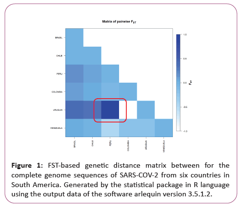
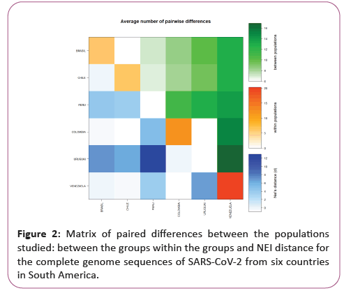
Genetic distance and molecular variation (AMOVA) analyses were not significant for the groups studied, presenting a variation component of 0.12 between populations and 4.46 within populations. The FST value (0.03) showed a low fixation index, with non-significant evolutionary divergences within and between groups, with a representative exception for haplotypes from Peru and Uruguai (Table 1) (Figures 1 and 2).
| Source of variation | DF | Sum of squares | Variance components | Percentage of variation |
|---|---|---|---|---|
| Among populations | 5 | 25.399 | 0.11704 Va | 2.56 |
| Within populations | 32 | 142.6 | 4.45630 Vb | 97.44 |
| Total | 37 | 168 | 4.57334 |
Fixation index FST: 0.02559
Significance tests (1023 permutations)
Va and FST: p (rand. value > obs. value)=0.30010, p (rand. value=obs. value)=0.00000, p-value=0.30010+0.01283
Table 1: Components of haplotypic variation and paired FST value for the 38 complete genome sequences of SARS-COV-2 from South America.
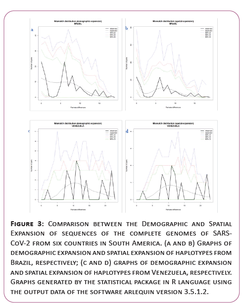
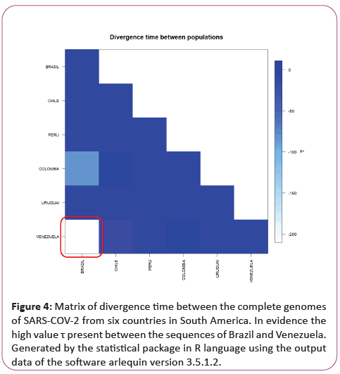
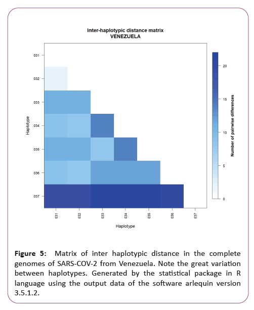
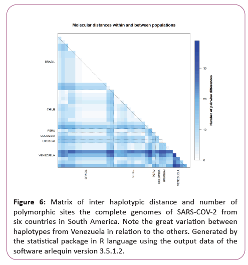
A significant similarity was also evidenced for the time of genetic evolutionary divergence among all populations; supported by T variations, mismatch analyses and demographic and spatial expansion analyses. With a representative exception for haplotypes from Venezuela (Table 2) (Figures 3-6).
Figure 3: Comparison between the Demographic and Spatial Expansion of sequences of the complete genomes of SARSCoV- 2 from six countries in South America. (a and b) Graphs of demographic expansion and spatial expansion of haplotypes from Brazil, respectively; (c and d) graphs of demographic expansion and spatial expansion of haplotypes from Venezuela, respectively. Graphs generated by the statistical package in R language using the output data of the software arlequin version 3.5.1.2.
Figure 4: Matrix of divergence time between the complete genomes of SARS-COV-2 from six countries in South America. In evidence the high value τ present between the sequences of Brazil and Venezuela. Generated by the statistical package in R language using the output data of the software arlequin version 3.5.1.2.
Figure 6: Matrix of inter haplotypic distance and number of polymorphic sites the complete genomes of SARS-COV-2 from six countries in South America. Note the great variation between haplotypes from Venezuela in relation to the others. Generated by the statistical package in R language using the output data of the software arlequin version 3.5.1.2.
| Statistics | BRASIL | CHILE | PERU | COLOMBIA | URUGUAI | VENEZUELA | Mean | s.d. | |
|---|---|---|---|---|---|---|---|---|---|
| Demographic expansion | Tau | 8.65821 | 3.41406 | 0 | 0 | 0 | 8 | 3.34538 | 4.08585 |
| Tau qt 2.5% | 1.43937 | 0 | 0 | 0 | 0 | 4.43744 | 0.97947 | 1.78922 | |
| Tau qt 5% | 2.76561 | 2.33788 | 0 | 0 | 0 | 5.36523 | 1.74479 | 2.17413 | |
| Tau qt 95% | 12.31057 | 17.19734 | 0 | 0 | 0 | 20.92787 | 8.40596 | 9.60534 | |
| Tau qt 97.5% | 13.72265 | 18.72268 | 0 | 0 | 0 | 21.95513 | 9.06674 | 10.27271 | |
| Theta0 | 0 | 4.28554 | 0 | 0 | 0 | 5.49999 | 1.63092 | 2.55563 | |
| Theta0 qt 2.5% | 0 | 0 | 0 | 0 | 0 | 0 | 0 | 0 | |
| Theta0 qt 5% | 0 | 0 | 0 | 0 | 0 | 0 | 0 | 0 | |
| Theta0 qt 95% | 1.82648 | 3.26617 | 0 | 0 | 0 | 12.13044 | 2.87052 | 4.72678 | |
| Theta0 qt 97.5% | 2.83189 | 4.79179 | 0 | 0 | 0 | 16.98018 | 4.10064 | 6.60932 | |
| Theta1 | 8.67921 | 13.59864 | 0 | 0 | 0 | 3414.9784 | 572.87604 | 1392.3517 | |
| Theta1 qt 2.5% | 3.11981 | 3.91268 | 0 | 0 | 0 | 27.98066 | 5.83553 | 10.98763 | |
| Theta1 qt 5% | 4.2627 | 4.56568 | 0 | 0 | 0 | 39.51658 | 8.05749 | 15.56301 | |
| Theta1 qt 95% | 33.99159 | 82.50502 | 0 | 0 | 0 | 323.1128 | 73.26823 | 126.61357 | |
| Theta1 qt 97.5% | 52.81974 | 162.02985 | 0 | 0 | 0 | 590.6107 | 134.24338 | 232.26574 | |
| SSD | 0.0433 | 0.0054 | 0 | 0 | 0 | 0.07165 | 0.02006 | 0.03041 | |
| Model (SSD) p-value | 0.3 | 0.99 | 0 | 0 | 0 | 0.04 | 0.22167 | 0.39418 | |
| Raggedness index | 0.07035 | 0.0086 | 0 | 0 | 0 | 0.1678 | 0.04112 | 0.06787 | |
| Raggedness p-value | 0.38 | 1 | 0 | 0 | 0 | 0.22 | 0.26667 | 0.39144 | |
| Spatial expansion | Tau | 6.18844 | 2.25056 | 0 | 0 | 0 | 8.24067 | 2.77994 | 3.60283 |
| Tau qt 2.5% | 1.28581 | 0.69166 | 0 | 0 | 0 | 3.44275 | 0.90337 | 1.34817 | |
| Tau qt 5% | 3.98499 | 1.97354 | 0 | 0 | 0 | 4.37483 | 1.72223 | 2.05513 | |
| Tau qt 95% | 10.32285 | 13.4485 | 0 | 0 | 0 | 14.53488 | 6.38437 | 7.12916 | |
| Tau qt 97.5% | 10.82249 | 17.56023 | 0 | 0 | 0 | 15.32114 | 7.28398 | 8.26907 | |
| Theta0 | 1.64652 | 4.96606 | 0 | 0 | 0 | 5.15534 | 1.96132 | 2.48474 | |
| Theta0 qt 2.5% | 0.00072 | 0.00072 | 0 | 0 | 0 | 0.00072 | 0.00036 | 0.0004 | |
| Theta0 qt 5% | 0.00072 | 0.00072 | 0 | 0 | 0 | 0.00258 | 0.00067 | 0.001 | |
| Theta0 qt 95% | 2.75007 | 7.34736 | 0 | 0 | 0 | 16.21983 | 4.38621 | 6.46833 | |
| Theta0 qt 97.5% | 3.02024 | 7.64974 | 0 | 0 | 0 | 20.05757 | 5.12126 | 7.90674 | |
| Theta1 | 2.30868 | 11.2256 | 0 | 0 | 0 | 8827.3024 | 1473.4728 | 3602.6287 | |
| Theta1 qt 2.5% | 0.82693 | 0.86722 | 0 | 0 | 0 | 20.59232 | 3.66398 | 8.30087 | |
| Theta1 qt 5% | 0.52435 | 1.18551 | 0 | 0 | 0 | 33.82173 | 5.97236 | 13.65272 | |
| Theta1 qt 95% | 12.86742 | 110.88566 | 0 | 0 | 0 | 2097.4888 | 370.20698 | 847.30175 | |
| Theta1 qt 97.5% | 15.34689 | 191.55404 | 0 | 0 | 0 | 5327.8721 | 922.46217 | 2159.5153 | |
| SSD | 0.02288 | 0.0056 | 0 | 0 | 0 | 0.07137 | 0.01664 | 0.02824 | |
| Model (SSD) p-value | 0.77 | 0.98 | 0 | 0 | 0 | 0.1 | 0.30833 | 0.44562 | |
| Raggedness index | 0.07035 | 0.0086 | 0 | 0 | 0 | 0.1678 | 0.04112 | 0.06787 | |
| Raggedness p-value | 0.68 | 1 | 0 | 0 | 0 | 0.22 | 0.31667 | 0.42641 |
Table 2: Demographic and spatial expansion simulations based on the τ, θ, and M indices of sequences of the complete SARS COV-2 genomes from six South American countries.
The molecular diversity analyses estimated per θ reflected a significant level of mutations among all haplotypes (transitions and transversions). Indel mutations (insertions or additions) were not found in any of the six groups studied (Table 3).
| Statistics | Brazil | Chile | Peru | Colombia | Uruguai | Venezuela | Mean | s.d |
|---|---|---|---|---|---|---|---|---|
| No. of transitions | 21 | 16 | 0 | 9 | 0 | 28 | 12.333 | 11.396 |
| No. of transversions | 7 | 2 | 0 | 3 | 0 | 14 | 4.333 | 5.391 |
| No. of substitutions | 28 | 18 | 0 | 12 | 0 | 42 | 16.667 | 16.428 |
| No. of indels | 0 | 0 | 0 | 0 | 0 | 0 | 0 | 0 |
| No. of TS sites | 21 | 16 | 0 | 9 | 0 | 28 | 12.333 | 11.396 |
| No. of TV sites | 7 | 2 | 0 | 3 | 0 | 14 | 4.333 | 5.391 |
| No. of subst. sites | 28 | 18 | 0 | 12 | 0 | 42 | 16.667 | 16.428 |
| No. of private subst. sites | 20 | 5 | 0 | 4 | 0 | 27 | 9.333 | 11.378 |
| No. of indel sites | 0 | 0 | 0 | 0 | 0 | 0 | 0 | 0 |
| Pi | 5.942 | 6.236 | 0 | 12 | 0 | 13.143 | 6.22015 | 5.6354 |
| Theta_k | N.A. | N.A. | N.A. | N.A. | N.A. | N.A. | N.A. | N.A. |
| Theta_k_lower | N.A. | N.A. | N.A. | N.A. | N.A. | N.A. | N.A. | N.A. |
| Theta_k_upper | N.A. | N.A. | N.A. | N.A. | N.A. | N.A. | N.A. | N.A. |
| Theta_H | N.A. | N.A. | N.A. | N.A. | N.A. | N.A. | N.A. | N.A. |
| s.d. Theta_H | N.A. | N.A. | N.A. | N.A. | N.A. | N.A. | N.A. | N.A. |
| Theta_S | 8.43824 | 6.14551 | 0 | 12 | 0 | 17.14286 | 7.28777 | 6.75543 |
| s.d. Theta_S | 3.34086 | 2.74879 | 0 | 8.83176 | 0 | 8.00564 | 3.82118 | 3.8262 |
| Theta_pi | 5.94167 | 6.23636 | 0 | 12 | 0 | 13.14286 | 6.22015 | 5.6354 |
| s.d. Theta_pi | 3.3517 | 3.6196 | 0 | 12.49 | 0 | 7.7307 | 4.532 | 4.83456 |
Table 3: Molecular diversity indices for the complete genomes of SARS-COV-2 from six countries in South America.
The D tests of Tajima and Fs de Fu showed disagreements between the estimates of general θ and π, but with negative and highly significant values, indicating, once again, an absence of population expansions (Table 4).
| Statistics | Brazil | Chile | Peru | Colombia | Uruguai | Venezuela | Mean | s.d. | |
|---|---|---|---|---|---|---|---|---|---|
| Ewens-Watterson test | Sample size | 16 | 11 | 1 | 2 | 1 | 7 | 6.3333 | 6.18601 |
| No. of alleles (unchecked) | 16 | 11 | 1 | 2 | 1 | 7 | 6.3333 | 6.18601 | |
| Observed F value | N.A. | N.A. | N.A. | N.A. | N.A. | N.A. | N.A. | N.A. | |
| Expected F value | N.A. | N.A. | N.A. | N.A. | N.A. | N.A. | N.A. | N.A. | |
| Watterson test: Pr(rand F <=obs F) | N.A. | N.A. | N.A. | N.A. | N.A. | N.A. | N.A. | N.A. | |
| Slatkin's exact test p-value | N.A. | N.A. | N.A. | N.A. | N.A. | N.A. | N.A. | N.A. | |
| Chakraborty's test | Sample size | 16 | 11 | 1 | 2 | 1 | 7 | 6.33333 | 6.18601 |
| No. of alleles (unchecked) | 16 | 11 | 1 | 2 | 1 | 7 | 6.33333 | 6.18601 | |
| Obs. homozygosity | 0 | 0 | 0 | 0 | 0 | 0 | 0 | 0 | |
| Exp no. of alleles | 8.13974 | 6.67071 | 0 | 1.92308 | 0 | 5.78902 | 3.75376 | 3.56148 | |
| p (k or more alleles) | N.A. | N.A. | N.A. | N.A. | N.A. | N.A. | N.A. | N.A. | |
| Tajima's D test | Sample size | 16 | 11 | 1 | 2 | 1 | 7 | 6.33333 | 6.18601 |
| S | 28 | 18 | 0 | 12 | 0 | 42 | 16.66667 | 16.42762 | |
| Pi | 5.94167 | 6.23636 | 0 | 12 | 0 | 13.14286 | 6.2201 | 5.6354 | |
| Tajima's D | -1.21891 | 0.06649 | 0 | 0 | 0 | -1.34385 | -0.41604 | 0.67194 | |
| Tajima's D p-value | 0.106 | 0.573 | 1 | 0 | 1 | 0.072 | 0.62517 | 0.44716 | |
| Fu's FS test | No. of alleles (unchecke) | 16 | 11 | 1 | 2 | 1 | 7 | 6.33333 | 6.18601 |
| Theta pi | 5.94167 | 6.23636 | 0 | 12 | 0 | 13.14286 | 6.22015 | 5.6354 | |
| Exp no. of alleles | 8.13974 | 6.67071 | 0 | 1.92308 | 0 | 5.78902 | 3.75376 | 3.56148 | |
| FS | 12.00112 | 6.00361 | 0 | 2.48491 | 0 | -1.0965 | -2.76939 | 5.31846 | |
| FS p-value | 0 | 0.002 | N.A. | 0.566 | N.A. | 0.184 | N.A. | N.A. |
Table 4: Neutrality tests for the complete genomes of SARS-COV-2 from six countries in South America.
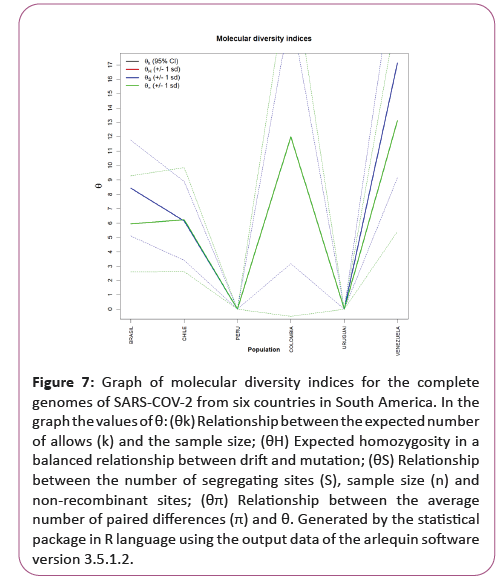
The irregularity index (R=Raggedness) with parametric bootstrap, simulated new θ values for before and after a supposed demographic expansion and in this case assumed a value equal to zero for all groups (Figure 7).
Figure 7: Graph of molecular diversity indices for the complete genomes of SARS-COV-2 from six countries in South America. In the graph the values of θ: (θk) Relationship between the expected number of allows (k) and the sample size; (θH) Expected homozygosity in a balanced relationship between drift and mutation; (θS) Relationship between the number of segregating sites (S), sample size (n) and non-recombinant sites; (θπ) Relationship between the average number of paired differences (π) and θ. Generated by the statistical package in R language using the output data of the arlequin software version 3.5.1.2.
Results and Discussions
As the use of phylogenetic analysis and population structure methodologies had not yet been used in this PopSet, in this study it was possible to detect the existence of 6 distinct groups for the complete genome sequences of SARS-CoV-2 from South America, but with minimal variations among all of them. The groups described here presented minimum structuring patterns and were effectively slightly higher for the populations of Brazil and Venezuela. These data suggest that the relative degree of structuring present in these two countries may be related to gene flow. These structuring levels were also supported by simple phylogenetic pairing methodologies such as UPGMA, which in this case, with a discontinuous pattern of genetic divergence between the groups (supports the idea of possible sub-geographical isolations resulting from past fragmentation events), was observed a not so numerous amount of branches in the tree generated and with few mutational steps.
These few mutations have possibly not yet been fixed by drift by the lack of the founding effect, which accompanies the behavior of dispersion and/or loss of intermediate haplotypes throughout the generations. The values found for genetic distance support the presence of this continuous pattern of low divergence between the groups studied, since they considered important the minimum differences between the groups, when the haplotypes between them were exchanged, as well as the inference of values greater than or equal to that observed in the proportion of these permutations, including the p-value of the test.
The discrimination of the 38 genetic entities in their localities was also perceived by their small inter-haplotypic variations, hierarchized in all covariance components: by their intra- and inter-individual differences or by their intra- and intergroup differences, generating a dendogram that supports the idea that the significant differences found in countries such as Brazil and Venezuela, for example, were shared more in their form than in their number , since the result of estimates of the average evolutionary divergence found within these and other countries, even if they exist, were very low.
Conclusion
Based on the high level of haplotypic sharing, tests that measure the relationship between genetic distance and geographic distance, such as the Mantel test, were dispensed in this Estimators θ, even though they are extremely sensitive to any form of molecular variation, supported the uniformity between the results found by all the methodologies employed, and can be interpreted as a phylogenetic confirmation that there is a consensus in the conservation of the SARS-CoV-2 genome in the Countries of America of America of South objects of this study, being therefore safe to affirm that the small number of existing polymorphisms should be reflected even in all their protein products. This consideration provides the safety that, although there are differences in the haplotypes studied, these differences are minimal in geographically distinct regions and thus it seems safe to extrapolate the levels of polymorphism and molecular diversity found in the samples of this study to other genomes of other South American countries, reducing speculation about the existence of rapid and silent mutations that , although they exist as we have shown in this work, they can significantly increase the genetic variability of the Virus, making it difficult to work with molecular targets for vaccines and drugs in general.
References
- Kumar S, Stecher G, Li M, Knyaz C, Tamura K (2018) MEGA X: Molecular evolutionary genetics analysis across computing platforms. Mol Biol Evol 35: 1547-1549.
- Excoffier L (2004) Patterns of DNA sequence diversity and genetic structure after a range expansion: Lessons from the infinite-island model. Mol Ecol 13: 853-864.
- Lewontin RC, Krakauer J (1973) Distribution of gene frequency as a test of the theory of the selective neutrality of polymorphisms. J Gen 74: 175-195.
- Rogers AR, Harpending H (1999) Population growth makes waves in the distribution of pairwise genetic differences. Mol Biol Evol 9: 552-569.
- Tamura K (1992) Estimation of the number of nucleotide substitutions when there are strong transition-transversion and G+ C-content biases. Mol Biol Evol 9: 678-687.
- Nei M (1987) Molecular evolutionary genetics. Columbia university press.
- Tajima F (1993) Measurement of DNA polymorphism. Mech Mol Evol 1: 37-59.
- Ewens WJ (1972) The sampling theory of selectively neutral alleles. Theor Popul Biol 3: 87-112.
- Paetkau D, Calvert W, Stirling I, Strobeck C (1995) Microsatellite analysis of population structure in Canadian polar bears. Mol Ecol 4: 347-354.
- Cavalliforza LL (1996) Population structure and human evolution. Proceedings of the Royal Society of London. Proc Royal Soc B 164: 362-379.
- Cockerham CC (1973) Analysis of gene frequencies. J Gen 74: 679-700.
- Excoffier L, Lischer HEL (2010) Arlequin suite ver 3.5: A new series of programs to perform population genetics analyses under Linux and Windows. Mol Ecol Res. 10: 564-567.
- Fu YX (1997) Statistical tests of neutrality of mutations against population growth, hitchhiking and background selection. J Gen 147: 915–925.
- Guy GP, Thomas CC, Thompson T, Watson M, Massetti GM (2015) Vital signs: melanoma incidence and mortality trends and projections MMWR. Morb and Mort Rep 64: 591-597.
- Pons O, Petit RJ (1995) Estimation, variance and optimal sampling of gene diversity. Theor Appl Genet 90: 462-470.
- Tajima F (1983) Evolutionary relationship of DNA sequences in finite populations. J Gen 105: 437-460.
- Excoffier L, Smouse PE, Quattro JM (1992) Analysis of molecular variance inferred from metric distances among DNA haplotypes: application to human mitochondrial DNA restriction data. J Gen 131: 479-491.
- Slatkin M, Hudson RR (1991) Pairwise comparisons of mitochondrial DNA sequences in stable and exponentially growing populations. J Gen 129: 555-562.
- Ray N, Currat M, Excoffier L (2003) Intra-deme molecular diversity in spatially expanding populations. Mol Biol Evol. 20: 76-86.
- Beaumont MA, Nichols RA (1996) Evaluating loci for use in the genetic analysis of population structure. Proceedings of the Royal Society of London. Proc Royal Soc B 263: 1619-1626.
- Slatkin M (1995) A measure of population subdivision based on microsatellite allele frequencies. J Gen 139: 457-462.
- Watterson GA (1975) On the number of segregating sites in genetical models without recombination. Theor Popul Biol 7: 256-276.
- Rohlf F (1973) Algorithm 76 hierarchical clustering using the minimum spanning tree. Comput J 16: 93-95.
- Watterson GA (1978) The homozygosity test of neutrality. J Gen 88: 405-417.
- Slatkin M (1994) An exact test for neutrality based on the Ewens sampling distribution. Gen Res 64: 71-74.
- Chakraborty R (1990) Mitochondrial DNA polymorphism reveals hidden heterogeneity within some Asian populations. Am J Hum Genet 47: 87-94.
- Tajima F (1989) Statistical method for testing the neutral mutation hypothesis by DNA polymorphism. J Gen 123: 585-595.
- Cockerham CC (1969) Variance of gene frequencies. Evol Lett 23: 72-83.
- Reynolds J, Weir BS, Cockerham CC (1983) Estimation of the coancestry coefficient: basis for a short-term genetic distance. J Gen 105: 767-779.
- Slatkin M (1996) A correction to the exact test based on the Ewens sampling distribution. Gene Res 68: 259-260.
- Nei M, Li WH (1979) Mathematical model for studying genetic variation in terms of restriction endonucleases. Proc Natl Acad Sci 76: 5269-5273.
- Gaggiotti OE, Excoffier LA (2000) Simple method of removing the effect of a bottleneck and unequal population sizes on pairwise genetic distances. Proc Royal Soc B 267: 81-87.
- Raymond M, Rousset F (1995) An exact test for population differentiation. Evol Lett 49: 1280-1283.
- Paetkau D, Waits LP, Clarkson PL, Craighead L, Strobeck C (1997) An empirical evaluation of genetic distance statistics using microsatellite data from bear (Ursidae) populations. J Gen 147: 1943-1957.

Open Access Journals
- Aquaculture & Veterinary Science
- Chemistry & Chemical Sciences
- Clinical Sciences
- Engineering
- General Science
- Genetics & Molecular Biology
- Health Care & Nursing
- Immunology & Microbiology
- Materials Science
- Mathematics & Physics
- Medical Sciences
- Neurology & Psychiatry
- Oncology & Cancer Science
- Pharmaceutical Sciences
