Keywords

Supply chain management; Just in time; Setup time; Processing time; Reduction waste

Introduction

In last couple of decades, JIT (Just in Time) systems frequently use in manufacturing industries to reduce the waste and increase the efficiency of overall systems. JIT system is not use only for reduction of waste but also use for the increase the efficiency and total quality of manufacturing processes. According to the Khan et al. there are several barriers faces during implementation of JIT system and mostly times companies are unable to respond or have limited capability to mitigate risks occurs during the implementation of JIT systems [1]. As per the research of Sarkar and Zangwill, [2] a stochastic cyclic manufacturing system where a machine processes n products in term one through n, and carry on this cycle every time.

Research Problem and Methodology

In the research of Takagi, waiting line model over system of polling, represents, a two item, product producing example: that reduction in setup times and reduction in processing time individually can upturn waiting time, however, work-in-process (via Law of Little) [3]. The existence of variation (variability) in processing times and set-up times are attributed for like a result of counterintuitive. For the system of the JIT (Just in Time) manufacturing, these results, findings are true for both approaches pull and push. In fact, some results, applications and interpretation are remains incomplete and somewhat mistaken, if we fail to perceive the following.

First of all, as per the little’s law, the conversion of waiting into number of units (physical) waiting in the system are known to be applicable in a push type system or conventional type system. In few system, manufacturing is planned in advance and then items are going through the machine centre(s) and then there physical queues are formed. Conversely, in a system of JIT of Pull the items, products cannot go themselves. In fact the demand occurs (for example: Kanban cards, multikaban systems etc.) according to the [4]. The system of Kanban might have to wait, but it might not be interpreted as a physical work-in-process buildup [4]. But that is such system’s novelty (Kanban system do not wait very long, however rational the system of JIT use “brute forces” like as lights to stop coming goods and thus break away from the cycle (continuous time). That happened when an unusually high level of variation exists, for example: breakdown of machines, etc. reasons of such systems shocks are then inspected to escape recurrence. However, no Work-in-Process (physical) build-up is possible, at least not because of above mentioned reasons).

Secondly, they assume in term to define their paradoxical results.

Var(d)-K_j(d_j)^aj (1)

for positive constants K_j, and they obtain:

W_i=(1-p_i)/2[d/(1-p)+hi_jXSIX{1+Var(S_j)/S)j₂+(1-p)K_j(d_j)ai/X_jS_jd}] (2)

Where j=1

where the setup time and unit processing time for product, i are assumed to be iid random variables with means d_i and Ss, and variances Var(d_i) and Var(S_i), respectively. Also, p_i=X_iS_i where X_i is the Poisson process parameter, p=E _i1-p_i and d=E _i1-d_i.

They then speculate that "clearly, if a_j<1, then W can increase without any bound”. We hope to debate that a_j cannot be in negative, i.e., reduction time in set-up does not increase variance of setup time. In the light of real world recommendations of Shingo examining in the JIT system [5], reduction of setup is actually accomplished through breaking down an original set of sequential activities into two main subsets of parallel activities external and internal setup. Although internal activities are those, which will be finished even machine is stopped, but external setup activities are not same like internal, these activities can be finished when the machine is in running operation. If setup is analysed like PERT network, then the critical path variances of a new reduced setup containing fewer activities provided and those actions and activities are independent must be smaller as compare to the variance of the original setup. In specific situations, by (1) and (2), then Cannot grow without bounds with decreasing d_j.

In addition, let rdj be the new setup reduced time with 0<r<1. By treading r as a decision variable, setup reduction team can manage and control, and definitely influence, the effect of setup reduction time on waiting time. It is very clear that the waiting time W_i will increase if,

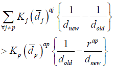(1)

To validate this in the case of 0<a_j<1, for S-Z example, let we replace their original variance of product 2 with Var

(d₂)=2305(d₂)0.5. So, for d₂=3, Var(d₂)(Unchanged)

~3992 (unchanged). So W₁=441, W₂=363

Now suppose that one product setup, d₂ is being targeted to be cut by 10%, 50%, 70%, and 100% (i.e., r=0.9, 0.5, 0.3, and 0). From condition (3), 14i will increase for a 10% or a 50% cut, and will decrease for a 70% or a 100% cut. The new waiting times will be W₁=444.9, 444.6, 415.4, and 1.125; W₂=363.1, 366.3, 365.9, 341.9, and 1.125, respectively, for 10%, 50%, 70% and 100% cuts. Waiting times first grew and then went down as we increased the amount of cut. Furthermore, an upper bound can be found by setting first derivative of Wi with respect to di to zero and solving for di, and plugging it into Wi. In this example, maximum W₁=449.48, maximum W₂=369.97, and both occur at d₂=2.025, i.e., at a cut of 32.67%. Furthermore, at a 55% cut (or, r=0.45) or beyond, both W₁ and W₂ drop below their respective original values of 441 and 363. A setup reduction management team could find this "good" r from condition (3), and use it for their planning purposes. Such criticality of choice of r value has not been stressed in earlier research.

When setup times for all products are cut by 100%, Var(d_j)=0 and d_j=0 V_j. In this case, however, the use of equation (2), we believe, will erroneously result in an infinite Wi. This is evident since by taking the limit of Var(d_j)->0 and d_j-O0V_j, Takagi (1986, p. 82) has shown that the explicit form of Equation (2).

For n=2 (see S-Z 1991, Eq. 2.2.8, p. 447) reduces to:

W₁= X₁E(S)/2(1-P₁)+(X_iP₂E(S₂) + 2(1-P)2 E(S₂))/2(1-P₂)(1-P₁-P₂) (1-P₁-P₂+2p1P₂)

W₂= X₂E(S₂)/2(1-P₂)+(X₂p₂E(S₂) + X(1-p₂)2E(S₂))/2(1-P₂)(1-P_i-P₂+2p₁P₂) (4)

Equation (4) comparison with Equation (2.2.8) [6] discloses that W_i is not just minimized in (4) but also is finite [7,8].

Conclusion

Lastly, it is important pointing out that Sarkar and Zangwill [2] used an extraordinary high Var(d₂)=3992, i.e., a 63.2 is standard deviation and a C.V of 63.2/3=2106%. After that, attribute the results of paradoxical to the presence of variance in processing time and set-up time distribution. However, this might not be right for all levels of variance. Such as; keeping everything else same in their example, if we only replace the setup time of product 2 by:

d₂=10/9 with prob 9/10

d₂=2 with prob 1/10

with d₂=1.2 and Var(d₂)=0.0711, the results are just the opposite. With processing times, S_i=S₂=1/50, we find that W₁=1.815 and W2=1.812; with a faster processing time, S_i=1/100 (while keeping S₂ fixed at 1/50), W14=1.799 and W₂=1.704. Both expected waiting times decreased. When setup time d₁ was reduced by 5% and 50%, W₁=1.759 and 142=1.757, and W₁=1.258 and W₂=1.254, respectively. Both decreased from their original values of 1.815 and 1.812, respectively. These results show that at a low level of variance, cutting setup or processing time does not necessarily increase waiting time.

In the mentioned, example vis-à-vis the Sarkar and Zangwill [2] claim (however reducing average processing time or set-up time) “if variances will not minimize proportionately arrivals will wait longer” the variance was, certainly, fixed. Although in our example does not fault their result of paradoxical, it does, since, determine a research need for characterization of variances ranges or processes for which reduction setup does not or does imply work in process reduction.

References

1. Khan SAR, Dong Q (2015) Case of civic company: The implementation of enterprise resource planning. International Business Research 8: 11.
2. Sarkar D, Zangwill WI (1991) Variance Effects in Cyclic Production System. Management Sci 37: 444-453.
3. Takagi H (1986) Analysis of Polling System. MIT Press, Cambridge, MA, USA.
4. Suzaki K (1987) The Manufacturing Challenge. The Free Press, New York, USA.
5. Shingo SA (1985) Revolution in Manufacture: The SMED System. Productivity Inc., Stanford.
6. Inman RA, Mehra S (1991) Just In Time (JIT). Applications for Service Environments.
7. Conway RW, Maxwell WM, Miller LW (1967) Theory of Scheduling. Addison-Wesley.
8. Cooper RB (1970) Queues Served in Cyclic Order: Waiting Times. The Bell System Technical J 49: 399-413.