Analysis of Imprecise Data: A Buy or Make Decision
1School of Economics and Management, Chang’an University, Xi’an, China
2School of Foreign Languages, Happy Home Foundation, Karachi, Pakistan
- *Corresponding Author:
- Syed Abdul Rehman Khan
School of Economics and Management
Chang’an University, Xi’an, China
Tel: 142455454414
E-mail: sarehman_cscp@yahoo.com
Received date: August 01, 2017; Accepted date: September 10, 2017; Published date: September 20, 2017
Citation: Khan SAR, Qianli D, Zhang Y, Khan SS (2017) Analysis of Imprecise Data: A Buy or Make Decision Glob Environ Health Saf. Vol. 1 No. 1:6.
Abstract
Since last couple of decades, make or buy decision becomes more critical. Because companies more focused on their core products and try outsource or buy items that are not very core for their products. While the manufacturing of an item or buy from the outside can be applied to a variety of decisions on the following: a new building, instruments need for the manufacturing of goods, equipment and tooling etc. This research paper mainly covers a buy or makes decision analysis involving imprecise data. We adopted the propagation of errors techniques to evaluate and check alternative (buy or make decision) with estimate errors. The examples of our numerical represent how the proposed error analysis creates more accurate discerning power. When assessing competing alternatives.
Keywords
Make or buy; Products; Decisions; Manufacturing; Analysis
Introduction
In today’s modern supply chain, make or buy decision is very important, somehow every company on certain point need to take decision about make or buy. While the manufacturing of an item or buy it from the outside can be applied to a variety of decisions on the following: a new building, parts, instruments need for the manufacturing of goods for sale, new equipment, tooling etc. infact the buy or make decisions are usually base on profitability and also depend on the firm’s financial position. While cost is usually not very important during make or buy decisions, but it somehow offer a good starting point. There are several significant issues involved during the decision of make or buy. First of all, the cost to production a product, item that is currently being bought can only be estimated. That estimation will vary upon the type of available data of cost, the activity level of the plant, treatment of overhead, and some other factors involved. But if there new facilities are to be bought, then the next question is: how depreciation is to be handled and what allowances need to be made for the training of manufacturing workers [1]. The market imperfections is the reason of unit cost of buying identical component, items to vary as well it is very hard to foresee when price of these items will be change over the period of time. That why it is not easy to predict exact cost values for buy or make analysis. Thus, conservative buy or make analysis, with somehow assumption might not be realistic.
There are various methods of conveying imprecise information. One approach is a bounded interval estimate, like (FC ± ΔFC) or [FC-ΔFC, FC+ΔFC] where FC is the fixed cost (estimated) and ΔFC is the probable error in FC. By Involving imprecise or interval input data, no technique has been applied to conduct buy or make decision analysis. This research paper will shows a decision rule in terms of make or precise discriminations among two competing substitutes expressed in rough ways. First, we will introduce the error technique “Propagation” and this captures the most likely aggregate error of a function owing to individual estimation errors. Second, we will show a simple make or buy model, which balances variable costs and fixed costs. Third, a relatively complex model by way of lot sizing method. The first model controls the minimum demand where the make option is preferred such as break-even point, as well the second model will determines the preferred choice with the given level of demand. An example (numerical) has been analysed for every model to shown the application of proposed method.
Propagation of Errors Technique
The objective of error analysis is to identify the Δy, mostly the probable error of the function y=f(x1, … , xn), when every variable xj have a bound interval of (xj ± Δxj) where Δxj is the error of estimation xj. We might consider two methods to obtain the composite error of Δy owing to individual errors Δxjs. One is the approach of approximation by the total differential; and the other is the approach of statistical by the error of propagation.
The error of composite has been defined, by using the total differential:
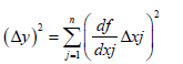 (1)
(1)
But it’s not definite whether the effect of every individual error is to decrease or increase the combined error which is a matter of randomness. And in simple words, we will at a loss to identify when to use either+Δxj or – Δxj. They might have same chances. Consequently the error composite Δy computed by total differential may render a much bigger amount than what it should be.
The other option of propagation error technique [2] resulted that the determination of the propagation of errors is to answer the question, “Give some set of numbers and them errors, what is the error in description function involving these numbers?” since the interval range of a distribution is comparative to its standard deviation, they gained the propagation errors of a function y = f(x1,… xn) by the statistical derivations:
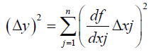 (2)
(2)
If we have a some special type of function like
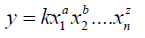 (3)
(3)
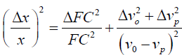
where, K is a constant and the fractional error in y is obtained by using equation 2:
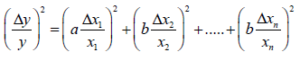 (4)
(4)
Now it can be supportable to restate our reasons for employing the error propagation instead of the total differential in the error analysis:
• We do not have to consider the direction of individual errors (i.e., +Δxj, –Δxj) because of the propagation of error equation (2) consists only of squares.
• The error of composite Δy which is calculated by equation (2) is always shorter than that by the total differential equation (1) because off the errors of opposite directions cancel each other internally. e.g., if we add two estimates (a ± Δa) and (b ± Δb) the error of composite calculated by equation (2) is (Δa2+Δb2)1⁄2, whereas its (Δa+Δb) by equation (2). Latest applications about propagation error techniques to decision analysis can be established in the research of [3,4].
Buy or make decision model 1
The first model conduct an analysis to identify whether make decision is more suitable or buy decision is more suitable when data of demand are not available. During the manufacturing an item in-house both costs occurred (variable and fixed). On the other side, buy components, item from supplier might avoid FC (fixed costs), but the per unit cost is typically higher than the per unit cost of manufacturing inside, in-house. The question is at what volume of output the item should be made rather than bought? That break-even point is the volume on which the total cost of “make” is equal to the total cost of “buy”. That is:
TCp=TCo
FC+VCp=VCo
FC+Vpx+vox
X=FC/(vo-vp)
Where, TCp=total cost of producing; TCo=total cost of buying; Vp=variable cost to produce one unit; Vo=purchasing price per unit.
When the parameters have estimates error like (FC ± ΔFC), (vp ± ΔVp) and (vo ± ΔVo), the find break-even point also own error like (x ± Δ x) per unit where the fractional error in X is attained by using equation (4).
The decision rule then becomes: if demand is much than (x+Δx) units, the most preferred option will be to “make”; and if demand is few, less than (x-Δx), the preferred option is to “buy”. And if demand is between the (x-Δx) and (x+Δx), then the decision is uncertain and fuzzy. So then we might look over other factors.
Numerical example: A component, item may be buy for $ (100 ± 5) per unit or produced within the manufacturing facility. The manager of plant estimates a FC (fixed cost of $ (300,000 ± 30,000) and VC (variable cost of $ (80 ± 4) per unit. What will be the minimum quantity to justify to the option of make?
Without considering estimate errors, the break even point is calculated as x=15,000 units. With errors estimation, the fractional error of x is as follows:
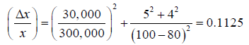
The amount of Δx is √0.1125x=5,031 units. The range of x is (15,000 ± 5,031) or [9,969, 20,031] units. Therefore, a quantity of 20,031 units or more units can justify to the “make” decision substitute in any situation.
For comparison purposes, the range of theoretical X is calculated. 30,000 units is the x maximum value, using $330,000 FC, vo=$105 and vp=$76. The minimum value of x is 9310 units using FC=$270,000, vo=$95 and vp=$84. The final results represents that the theoretical range of x is larger than the range obtained by the propagation of errors technique. In simple words, this technique concentrates more practical range of future results, outcomes.
Buy or make decision model 2
Irrespective of our decision of buy or make, we neither buy nor make all items, components at once. If we buy the per year demand can be fulfilled by a FO (fixed order) quanity, which can be resolute by EOQ (economic order quantity) analysis.
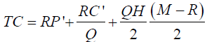
Total cost per year=(Purchase Cost+Holding Cost+Order Cost)
The optimal lot size Q0 is determined by
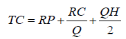
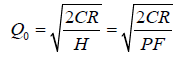
Where, R=annual demand in units; P=purchasing cost of an item; C=ordering cost per order; F=annual holding cost as a fraction of unit cost; H=PF=holding cost per unit per year.
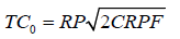
When the optimum lot size Q0 is utilized in the decision of order then the minimum total inventory cost will be obtained by:
If component, items are internally manufactured; the production quantity can be attained from EPQ (economic production quantity) analysis.
Total Annual Cost=Production Cost+Holding Cost+Set-up Cost
The economic production quantity is determined by
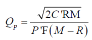
Where, R=annual demand in units; P'=unit production cost; M=annual production capacity in units; C'=set-up cost per production run; H=P'F=holding cost per unit per year; F=annual holding cost as a fraction of unit cost.
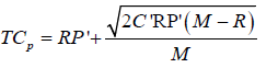
Once the economic manufacturing quantity is utilized in the manufacturing decision, the Total minimum annual cost is attained by:
According to the Tersine [5] a comparison of the make analysis (EPQ) with the buy analysis (EOQ) can decide the most desirable economic alternative. This is, TC0>TCp.
Choose the make option when the parameters are expressed in an rough way like (R ± ΔR), (P ± ΔP), (C ± ΔC), and (F ± ΔF), the propagation of errors in TCo is attained by:
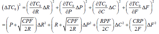
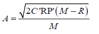
This propagation of errors in TCp with imprecise input is then obtained by:
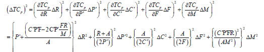
Where:
While the cost ranges may be expressed by (TCo ± ΔTCo) and (TCp ± ΔTCp). The rule of decision under rough information is given as: choose the option of “make” if (TCo-ΔTCo)>(TCp-ΔTCp).
Example from numerical: A component item might be bought for $25 one unit or produced at 10,000 rates annually for $23 per unit. If purchased, the order cost will be 5 dollar, compared with 50 dollar of set up cost for production. The demand of per year for the item is 2500 units; as well the cost of holding is 10%. Should the item, component be manufactured internally or purchased externally?
TCo=$62,750 and TCp=$58,157. The component, item should be produced meanwhile this is the least cost alternative.
If we expect 10% error estimation (e.g., ΔC/C=ΔR/R=0.1) in all parameters of total inventory formulas, we attain the ranges of total cost of two given options:
TCo=$[53,893, 71,607] and TCp=$[49,992, 66,320].
These two options have an area of overlapping, which implies that “buy” option has some chance of being more cheaply than the “make” option.
We have conducted a sensitivity analysis with different error of estimates mentioned in the Table 1 and also represented in Figure 1. If the error will be more than 2.7%, an overlap between options begins to occur. In simple words, in our example of numerical “make” option is always preferred when the error is small than 2.7%.

Figure 1: Total cost ranges of buy or make with errors estimate.
| Input error levels (%) | Make (TCp ± ∆TCp) | Buy (TC0 ± ∆TC0) | Probability of ‘’buy’’ preferred (%) |
|---|---|---|---|
| 0 | 58,157 | 62,750 | 0 |
| 1 | [57,340,58,972] | [61,864,63,636] | 0 |
| 2.7 | [55,952,60,361] | [60,358,65,141] | 0 |
| 5 | [54,075,62,239] | [58,321,67,178] | 10.6 |
| 10 | [49,992,66,320] | [53,893,71,607] | 26.7 |
| 20 | [41,829,74,484] | [45,036,80,463] | 37.5 |
| 30 | [33,666,82,648] | [36,180,89,320] | 41.5 |
Table 1: Total cost ranges of buy and make with different error of estimates.
In the table, last column presented the probability that current unfavourable “buy” decision is preferred to the favourable “make” decision. That is the probability that the cost of “make” is more than the “buy” option. e.g., with 10% error rate the “buy” option has a 26.7% chance of being the preferred alternative using the formula mentioned in the Appendix.
When there will be an overlap between the two costs, we might have to focus towards other factors (e.g., non financial) some factors included; reliability of the quality and quantity of supply, idle plant capacity, in house capabilities, workforce stability [1,5] the Various different criteria for decision analysis under imprecise information.
Conclusion
The selection of options or decision regarding manufacturing or buying product from outside may play a significant role on the long-term as well in daily operations of a company. But mostly input cost data need to be estimated in advance. When forecasting future cash outcomes so an error estimate may not be avoided. While the conservative approach about buy or make decision with certainty assumptions cannot be realistic. The bounded interval estimate is one common allowance scheme to compensate for the inherent error estimating. In the study, we have applied the propagation of errors techniques to check and evaluate alternatives (buy or make decisions) with estimate errors. The examples of numerical; presents how the proposed error analysis generates more accurate discerning power. When assessing competing alternatives.
References
- Gambino AJ (1980) The Make or Buy Decision. National Association of Accountants, New York, USA.
- Pugh EM, Winslow GH (1966) The Analysis of Physical Measurements. Addison-Wesley, Reading, MA, USA.
- Yoon KP (1990) Capital investment analysis involving estimate error. The Engineering Economist 36: 21-30.
- Yoon K, Kim G (1989) Multiple Attribute Decision Analysis with Imprecise Information. IIE Transactions 21: 21-25.
- Tersine RJ (1989) Principles of Inventory and Material Management. North-Holland, New York, USA.

Open Access Journals
- Aquaculture & Veterinary Science
- Chemistry & Chemical Sciences
- Clinical Sciences
- Engineering
- General Science
- Genetics & Molecular Biology
- Health Care & Nursing
- Immunology & Microbiology
- Materials Science
- Mathematics & Physics
- Medical Sciences
- Neurology & Psychiatry
- Oncology & Cancer Science
- Pharmaceutical Sciences