Keywords
Chickpea, genotype × environment interaction, combined analysis of variance, GGE Biplot
Introduction
Chickpea (Cicer arietinum L.) is Iran's most important food legume crop, comprising nearly 64% of the area grown
to food legumes in the country [1,21]. Chickpea is grown on 700,000 ha in Iran and ranks fourth in the world after
India, Pakistan and turkey [2]. The agricultural sector of Iran is attempting to improve high yielding chickpea
genotypes with identification and introducing of stable and adaptive cultivars [3, 4]. However, high yield is often
associated with decreased yield stability [5]. The terms 'stability' or 'adaptability' refer to consistent high
performance of genotypes across diverse sets of environments [6]. In order to identify the most stable and high
yielding genotypes, it is important to conduct multi-environment trials [7]. Genotypes tested in different
environments often have significant fluctuations in yield due to the response of genotypes to environmental factors
[8]. These fluctuations are often referred as genotype × environment interaction (GEI). The methods used for
evaluation of GEI and stability performance can be classified into two groups: graphical (GGE biplot and
performance plots) and non-graphical [parameric (univariate and multivariate) and non-parameric].
The yield of each cultivar in each test environment is a mixture of environment main effect (E), genotype main
effect (G) and genotype × environment interaction (GEI). Moreover, G and GE must be considered simultaneously
when making cultivar selection decisions. For this reason , instead of trying to separate G and GE, Yan et al. [9]
combined G and GE and referred to the mixture as GGE. Yield data from regional performance trials, or more
generally, multi environment trails (MET), are usually quite large, and it is difficult to understand the general pattern
of the data without some kind of graphical presentation. The biplot technique [10] provides a powerful solution to
this problem. A biplot that displays the GGE of a MET data, referred to as a GGE Biplot (graphical method), is an
ideal tool for MET data analysis [11, 12]. In analyzing Ontario winter wheat performance trial data, Yan and Hunt
[13] used a GGE biplot constructed from the first two principal components (PC1 and PC2) derived from PC analysis
of environment- centered yield data. GGE biplot can be useful in two major aspects. The first is to display the
which- won – where pattern of the data that may lead to identify high- yielding and stable cultivars and
discriminating the representative test environments [12].
The objectives of this study were (i) to interpret G main effect and GE interaction obtained by combined analysis of
yield performances of 20 chickpea genotypes over eight environments (ii) application of the GGE biplot technique
to examine the possible existence of the different mega- environments in chickpea- growing regions and (iii)
visually assess how to vary yield performances across environments based on the GGE Biplot.
Materials and Methods
Plant materials
In order to identify stable and high performance genotypes of chickpea (Table 1) a randomized complete block
design (RCBD) with three replications was carried out in two different environments (rainfed and irrigated) for four
growing seasons (1387-1390) (8 environments E1 to E8) in the Campus of Agriculture and Natural Resources of
Razi University of Kermanshah, Iran (47° 20′ N, 34° 20′ E and 1351 m above sea level). The maximum and
minimum temperatures were 44°C and –27°C and the average rainfall was 478 mm. The soil of experimental field
was clay loam with pH7.1.
Table 1: The codes and names of chickpea genotypes
Each plot consisted of five rows of 1.5 meter length. Row to row and hill-to-hill distances were kept at 30 and 10
cm, respectively. Data on seed yield were taken from the middle three rows of each plot. At harvest seed yield was
determined for each genotype at each test environments.
Statistical analysis
Analysis of variance was conducted by SAS, software to determine the effect of environment (E), genotype (G) and
GE interaction. The first two components resulted from principal components were used to obtain a biplot by GGE
biplot software [11]. The basic model for a GGE biplot is :
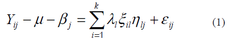
Where  the mean yield of genotype i(=1,2,…,n) in environment j(=1,2,…m), μ = the grand mean,
  the
main effect of environment j,
the
main effect of environment j,  being the mean yield of environment j,
 the singular value (SV) of lth
principal component (PC), the square of which is the sum of squares explained by PCl=(l=1,2,…,k with k≤ min
(m,n) and k=2 for a two- dimensional biplot),
the singular value (SV) of lth
principal component (PC), the square of which is the sum of squares explained by PCl=(l=1,2,…,k with k≤ min
(m,n) and k=2 for a two- dimensional biplot),  the eigenvector of genotype i for PCl,
 the eigenvector of
environment j for PCl,
the eigenvector of
environment j for PCl,  the residual associated with genotype i in environment j.
To generate a biplot that can be used in visual analysis of MET data, the SVs have to be partitioned into the
genotype and environment eigenvector so that the model (1) can be written in the form of 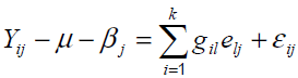 where gil and elj are called PCl scores for genotype i and environment j,
respectively. In a biplot, genotype i is displayed as a point defined by all gil values, and environment j is displayed as
a point defined by all elj values (l=1 and 2 for a two- dimensional biplot) [14].
where gil and elj are called PCl scores for genotype i and environment j,
respectively. In a biplot, genotype i is displayed as a point defined by all gil values, and environment j is displayed as
a point defined by all elj values (l=1 and 2 for a two- dimensional biplot) [14].
Results and Discussion
According to the results of combined analysis of variance (Table 2), genotype ×environment interaction was highly
significant for grain yield indicating that we can proceed and calculate phenotypic stability. GGE biplot was
constructed using the first two principal components (PC1 and PC2) derived from subjecting the environmentcentered
data to singular-value decomposition [15]. Results of GGE biplot also showed that the first two principal
components (PC1 and PC2) justified 68% of the sum of squares with PC1= 40.5% and PC2= 27.5% of the GGE sum
of squares. GGE biplot graphically displays G plus GE of a MET in a way that facilitates visual cultivar evaluation
and mega- environment identification [9]. Only two PC (PC1 and PC2) are retained in the model because such a
model tends to be the best model for extracting patterns and rejecting noise from the data. In addition, PC1 and PC2 can be readily displayed in a two dimensional biplot so that the interaction between each genotype and each
environment can be visualized [14].
Table 2: Combined analysis of variance over eight environments
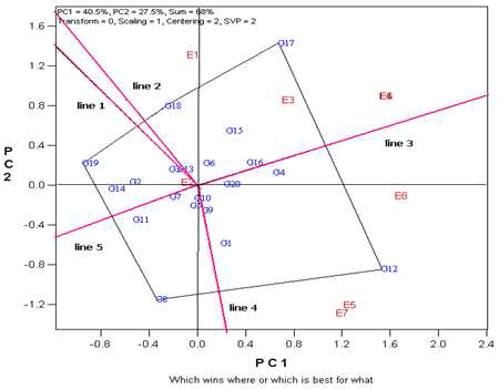
Winning Genotype and Mega-environment
Visualization of the “which-won-where” pattern of MET data is important for studying the possible existence of
different mega-environments in a region [9, 12] (Figure 1). The polygon view of a biplot is the best way to visualize
the interaction patterns between genotypes and environments and to effectively interpret a biplot [16]. The vertex
genotypes in this investigation were G8, G12, G17 and G19. The vertex genotype for each sector is the one that gave
the highest yield for the environments that fall within that sector. Another important feature of Figure 1 is that it
indicates environmental groupings, which suggests the possible existence of different mega-environments. Thus,
based on biplot analysis of 8 environments of data, three mega-environments are suggested in Figure 1. The first megaenvironment
contains environments E1, E3, E4 and E6, with genotype G17 (X96TH41K4) being the winner; the
second mega environment contains environments E5, E7 and E8, with genotype G12 (X96TH46) being the winner.
The environment of E2 makes up another mega-environment, with G19 (FLIP-82-115) the winner.
Figure 1: polygon views of the GGE biplot based on symmetrical scaling for the which-won-where pattern of genotypes and environments
Mean Performance and Stability of Genotypes
In (Figure 2) the average tester coordinate (ATC X-axis) or the performance line passes through the biplot origin with
an arrow indicating the positive end of the axis. The ATC Y-axis or the stability axis passes the plot origin with
double arrow head and is perpendicular to the ATC X-axis. The average yield of the genotypes is estimated by the
projections of their markers to the ATC X-axis [17]. Genotypes 12 and 17 had the highest mean yield and genotype
19 had the poorest mean yield. Mean yields of the genotypes were in the following order: G12 > G17 > G4 > G16 > G15 > G20 > G6= G1. The performance of genotypes G12 and G17 were the most variable (least stable), whereas
genotypes G4, G16 and G20 were highly stable with high grain yield.
Figure 2: Average environment coordination (AEC) views of the GGE biplot based on environment- focused scaling for the means performance and stability of genotypes.
Ranking genotypes relative to the ideal genotypes
An ideal genotype is one that has both high mean yield and high stability. The center of the concentric circles (Figure
3) represents the position of an ideal genotype, which is defined by a projection onto the mean-environment axis that
equals the longest vector of the genotypes that had above-average mean yield and by a zero projection onto the
perpendicular line (zero variability across environments). A genotype is more desirable if it is closer to the ideal
genotype. Although such as ideal genotype may not exist in reality, it can be used as a reference for genotype
evaluation [18].
Figure 3: GGE biplot based on genotype – focused scaling for comparison. The genotypes with the ideal genotype.
Because the units of both PC1 and PC2 for the genotypes are the original unit of yield in the genotype-focused
scaling (Figure 3), the units of the AEC abscissa (mean yield) and ordinate (stability) should also be the original unit of
yield. The unit of the distance between genotype and the ideal genotype, in turn is the original unit of yield as well.
Therefore, the ranking based on the genotype-focused scaling assumes that stability and mean yield are equally
important [19]. Therefore, genotypes G4 and G12 which fell into the center of concentric circles, were ideal
genotypes in terms of higher yield ability and stability, compared with the rest of the genotypes. In addition G15, G16 and G17 located on the next concentric circle, may be regarded as desirable genotypes.
Ranking environment relative to the ideal environment
The GGE biplot way of measuring representativeness is to define an average environment and use it as a reference
or benchmark. The average environment is indicated by small circle (Figure 4). The ideal environment, represented by
the small circle with an arrow pointing to it, is the most discriminating of genotypes and yet representativeness of
the other tests environments.
Figure 4: GGE biplot based on environment-focused scaling for comparison the environments with the ideal environment.
Therefore, E8 was the most desirable test environment followed by E4 and E6
Figure 5 is the same GGE biplot as (Figure 4) expect that it is based on environment–focused scaling [19]. This type of
AEC can be referred to as the "Discriminating power vs. Representativeness " view of the GGE biplot. it can be
helpful in evaluating each of the test environments with respect to the following questions: [20].
Figure 5: GGE biplot based on discriminating power and representativeness of the test environment.
1. is the test environment capable of discriminating among the genotypes, i.e., does it provide much information
about the differences among genotypes?
2. Is it representative of the mega-environment?
3. Does it provide unique information about the genotypes?
Thus E8 may be regarded as an ideal test environment and E4, E6, may constitute a next set of test environments if
the pattern shown in (Figure 5) is repeatable across years.
References
- Sabaghpour SH, Sadeghi E, Malhotra RS, 2003. Int. chickpea conf, Raipur. India.
- FAO, 2001. UN food and Agriculture organization. Rome, Italy.
- Ebadi Segherloo A, Sabaghpour SH, Dehghani H, Kamrani M, 2010. Plant breed and crop Sci. J, 9: 286-292.
- Rozrokh M, Sabaghpour SH, Armin M, Asgharipour, 2012. Euro. J. Exp. Bio, (6):1980-1987.
- Padi K, 2007. J. Agri. Sci, 142: 431-444.
- Romagosa I, Fox PN, 1993. In: Hayward, M.D., Bosemark, N.O., Romagosa, I. (Eds.), Plant Breeding: Principles and Prospects. Chapman & Hall, London, pp. 373-390.
- Lu'quez JE, Aguirreza LAN, Aguero ME, Pereyra R, 2002. Crop Sci, 188: 225.
- Kang MS, 1993. Agron. J, 85: 754-757.
- Yan W, Hunt LA, Sheng Q, Szlavnics Z, 2000. Crop Sci, 40: 597-605.
- Gabriel KR, 1971. Biometrika, 58: 453-467.
- Yan W, 2001. Agron. J, 93:1111-1118.
- Yan W, Cornelius PL, Crossa J, Hunt LA, 2001. Crop Sci, 41:656-663.
- Yan W, Hunt LA, 2001. Crop Sci, 41:19-25.
- Yan W, Hunt LA, 2002. Crop Sci, 42: 21-30.
- Farshadfar E, Zali H, Mohammadi E, 2011. Annals of Biol Res, 6: 282-292.
- Yan W, Kang MS, 2003. GGE biplot analysis: A graphical tool for breeders, geneticists, and agronomists. CRC Press, Boca Raton, FL.
- Amin K UR, Rahman H, Rahman N, Arif M, Hussain K, Iabal MH, Afridi KH, Sajjad M, IshaQ M, 2011. Agric.J, 27.
- Yan W, Tinker NA, 2006. Can. J. Plant Sci, 86: 623-645.
- Yan W, Rajcan I, 2002. Crop Sci, 42:11-20.
- Morris CF, Campbell KG, King GE, 2004. Plant Genet. Res, 2:59–69.
- Rasaei1 B, Ghobadi1 ME, Ghobadi2 M, Abdollah Nadjaphy A, Rasaei1 A, 2012. Euro. J. Exp. Bio, 2 (4):1113-1118.