European Journal of Experimental Biology Open Access

Keywords

Environmental Effects, Economic Growth, Energy Consumption

Introduction

Attention to sustainable development currently, the not only has been necessary in all areas of social, cultural and especially economic, but disregarding the criteria influence on sustainable development, the cost of irreparable does for each community. On this basis one of the influential factors in imposing social costs, implementation plans is based on scientific rectifier based foreign material interests and social and environmental considerations. For example assessment most plans and projects is more focused on the economic costs and benefits and investment return period much attention is not costs and social benefits and important environmental the estimated total amount of costs and benefits. Purpose In this paper the expression patterns conventional economic theory and methods of assessment and environmental projects, is introduced an integrated strategy for economic environmental. Nowadays the relationship between economic growth and environmental quality as Inverted U is know to environmental Kuznets [1] Curve. Now that in the early years of economic growth, it is increases the amount of environmental degradation, but over time after reaching a certain level of growth, improved environmental quality. In other words, High-growth stages will reduce the amount of environmental degradation. This study wills economic impact on air pollution in the environmental Kuznets [1] Curve hypothesis (the relationship between economic growth and the environment).

In this regard, in addition knowledge of the structure and shape of the curve, also will review some of the factors affecting the environment. For example can be said in time to achieve high economic growth, increases literacy level and knowledge of citizens and people react to their and they protest against air pollution or economic growth, technology advances more is used in the production process and therefore less pollution is created in the production process [2]. On the other hand in communities where have reached high level of growth, is serious discusses the measurement and control (monitoring) of pollution and continuous contamination is reflected indicators and in the media and public opinion show sensitivity to it. So, against pollution and generally sources of pollution protests come from Non Government organizations. In these communities, the situation has been runs strongly numerous environmental laws and learning. Some governments on polluting activities, environmental fines imposed, or has stopped polluting activities to or the manufacturer are forced to using filters and devices to reduce pollution. In other words, having them to pollution internalize. The relationship between economic growth and environmental quality in a duration Long-term can be directly, reverse or a combination of both. This discussion (The relationship between economic growth and environmental quality) has been subject of many studies. If we examine the formation of these field studies, It suggests that during recent decades, both the general intellectual there is in this area that eventually have become a third approach.

The first approach a checks to option between economic growths and maintain environmental standards, this means that economic growth and thus increased production and consumption, whether or not are need ingredients and more energy as a second-generation data and mutually with increase in waste production [3]. In other words, during the process of economic development increases Income levels, more in the extraction of natural resources and increased environmental destruction, human welfare reduced. Therefore, growth in economic activity considered a risk in this respect. So be argued that policymakers in this connection should take a choice, namely with the aim of achieving higher economic growth, be receptive environmental hazards more or if belief in the necessity to preserve the environment should give consent to very low levels economic growth that is difficult choice. On the other hand, this spectrum, there is second approach. In this group is believed to the improvement environmental quality is parallel to economic growth to environmental standards should went in the current economic growth. Because higher level of income, the demand is for product uses the lower level of raw materials (Less material intensive), also the revenue is the Increase demand for environmental quality and this is means acceptance criteria and terms of protection environmental.

The third approach that raised from the early 90s, between economic growth and environmental pollution a relationship has been as Inverted U that this known the hypothesis transfer of environmental or environmental Kuznets curve hypothesis, the relationship his name is of Simon Kuznets [1], Nobel laureate between income inequality and income and found a relationship as Inverted U. So Kuznets curve hypothesis, in the early stages of economic growth, is high environmental degradation until this be up to a point in their and then in the process of growth, improved environment.

Economic growth and impacts of environmental biology: In economic theory, the relationship between economic growth and environmental quality was raise in environmental Kuznets hypothesis (EKC). Based on EKC, time that a country develops, beginning began to increase pollution but after reaching a certain level of economic development reduced pollution. In fact, it was inevitable environmental degradation at the beginning stage of economic growth and that is a country in the early stage of development is inevitably of environmental degradation to develop. However, after reaching a sufficient level of economic development, the importance of issues of sustainable development and environmental issues and with efforts to prevent environmental degradation, economic growth achieved with less pollution. It stated that there is relationship U reverse between economic growth and environmental pollution is that the same environmental curve Kuznets [4].

Energy consumption and impacts of environmental biology: Maier & Kent the relationship between energy consumption and environmental degradation are expressed that this although the after the industrial revolution particularly in recent decades with the use of energy, increased the average productivity of production factors and but use contaminant effects your energy, caused environmental degradation. Because main greenhouse gases published in as carbon dioxide is the result of use of fossil fuels. Hence, energy sector has the highest share change in environmental issues and so are closely together energy policy and policy environment [5].

Population and impacts of environmental biology: In the literature economic environment, physical society considered another factor the pollutant environment. Because with increasing population, increased demand for agricultural land, energy resources, and water resources etc. This is followed destruction of forests and pastures, loss of land fertility fertile agricultural land and pollution environment. Many researchers of this matter studies have been by using Statistics and time series data and cross a number of developed countries and level world. Research results show that human factor and population growth considered important factor increasing environmental pollution [6]. About the relationship between urban population and environmental pollution, there are two different perspectives. The first view points out that Influence increase in urban population is positive on environmental pollution, because with increasing urbanization increases use infrastructure, transport and energy transfer of agricultural industry causes increased environmental pollution. However, the second view emphasizes that urban culture makes energy makes energy in cities be more efficient the villages and reduced pollution. The relationship between urban population growth environmental pollution can be positive or negative [7].

About information and environmental impact data, it has been used information and data from the research of green GDP done by honest and wise in 2001. Researchers in this study levels of environmental depreciation is calculated by honest and wise have the as indicators of environmental impact. Now because have overview on behavior these three variables, namely economic growth, population growth and environmental impacts, long-term process of moving them is displayed in Figure 1 during 1346-1380. A glimpse to the chart shows that process temporal changes P, has been an upward trend and has had a constant process. So, neither of these two, behavior does not consistent with theory investigated. But LGDPP beginning has the an incremental step and ascending and after reaching to peak, will begin to reduction that is adapted theory. This type of behavior LEI is evident somewhat.

Another factor that called about source and source of environmental impact is economic growth. Increase economic growth, makes intensive use of natural resources on the other hand, undesirable outputs also is effective in destroying the environment. In this context, many studies have done that among them, could named of the environmental Kuznets curve. According to this theory, in the early stages growth and development (at this stage is low levels of incomes and growth) with rising per capita income, also increased rate of environmental degradation. The incremental process economic growth continues along with increasing environmental destruction and damage, until after some reaches its peak, then if economic growth again to continue then not only does not increase environmental side effects but also, will decrease strongly.

The first study by Grossman and Krueger [8] been done it is the story of existence and form such a relationship as Inverted U, between these two variables. Shafik and Bandyopathyay [9], in this context, using time series data, experimental studies have done that Grossman and Krueger [8] confirmed the theory on environmental Kuznets curve (EKC) [10]. Shafik and Bandyopathyay [9] in another study, in 1994 using large volumes of data to countries (Which are located in a variety of development) form reverse has gained for particulate in air (SPM) and sulfur dioxide, SO2. He the average income turning point for the SO₂ is estimated figure about $3,000. Roca and et. al. [11], recent theory the review for several important air pollutants, for Spain and such conclusions have the SO₂ emissions is compatible Kuznets with ecological theory. However, the other pollutants the match and consistent there is not with the above theory. General all empirical studies shows that a form inverted U there is between standards of environmental degradation and real per capita income without to note existing mechanism for to the creation such phenomena. Experimental results of many studies to confirm existence Kuznets curve the environmental for some air pollutants like Suspended particles in air, Sulfur dioxide SO2 but, in the case of CO₂ and water pollutants the results varied is obtained based on existence or absence such a relationship [12].

So briefly, can reasons and mechanisms to reduce emissions by income growth and economic growth (Theory EKC) named in the following format: A) Quality and improve the environment, from the perspective of microeconomics, is a luxury item. Therefore, at high income levels are requested and increasing income levels, reduced publication pollutants. B) Changes in the composition of manufactured goods and especially towards a service, economy followed less pollution. C) Improvements in production techniques brings high economic growth and less pollution [11].

Materials and Methods

Model: As noted earlier, the purpose of these articles is survey environmental impact energy and economic growth in Iran. In this regard, literature of subject points out that level of environmental impact Depends on To Per capita income (economic growth), energy and population growth. In this model from the pattern of per STIRIPAT and is based on the empirical studies, it is especially the study Alam et. al. [7] stipulated that as follows.

CO₂ f (EI ,GDPP ,URBN , RPOP )

(1)

In the above equation CO2 marker emissions per capita carbon dioxide (Based on meter - tons) GDP per capita fixed price year 1376 (Billion riyals) , EI energy intensity (In terms of equivalent Barrels of crude oil), RPOP population growth rate, URBN urban population (Per thousand people), B₁ to B₂ dependent variable tension than explanatory variables e_t is random disturbance term.

Methodology: Generally a STAR model for a univariate time series y_t observed in t = 1 - p, 1 - (p-1),…, -1, 0, 1, …, T - 1, T is defined as follows:

(2)

Where:

y_t = The variable of interest, bi and b*_i i = 0, 1... p = Autoregressive parameters

F (S_t) = A transition function allowing the model to switch smoothly between regimes which is bounded by zero

u_t = A random error component believed to satisfy the assumption u_t ~ iid(0,s² )

The model in Eq. 2 can estimated if the null hypothesis of constancy in parameters rejected. This estimated model might provide information about where and how the parameters change. It is important to have the STR model in (2) as the alternative hypothesis to the null. Two forms of the transition functions given in Terasvirta are the logistic function:

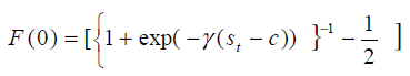(3)

And the exponential function:

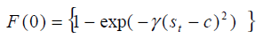(4)

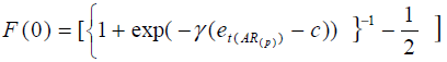
A third re-parameterized version of (2) proposed by Liew and et. al. [13] the Absolute Logistic transition function is:

(5)

Our model is:

(6)

The LSTAR model describes an asymmetric realization, that is, this model can generate one type of dynamics for increasing growth rate of inflation and another for reductions of the rate of inflation. The objectives of this study are First, to evaluate the forecasting performances of LSTAR, ESTAR, ALSTAR models. Second, we shall evaluate our proposed ELSTR model using the AR, LSTAR and the ALSTAR models as benchmark. We shall accomplish this task by investigating the Mean Square Error (MSE) and the robustness of this criterion subjected to Meese and Rogoff [14] test.

Results and Discussion

Unit Root Test: We use the Augmented Dickey-Fuller (1979) t-statistic when to difference time series data to make it stationary. Here are the various cases of the test equation:

A. When the time series is flat (i.e. does not have a trend) and potentially slow turning around zero, we use the following test equation:

(7)

Where the number of augmenting lags (p) determined by minimizing the Schwartz Bayesian information criterion or minimizing the Akaike information criterion or lags dropped until the last lag is statistically significant. Mifrofit allows all of these options to choose. This test equation does not have an intercept term or a time trend. Unfortunately, the Dickey-Fuller t-statistic does not follow a standard t-distribution as the sampling distribution of this test statistic skewed to the left with a long, left-hand-tail. Microfit will give us the correct critical values for the test, however. Notice that the test is left-tailed. The null hypothesis of the Augmented Dickey-Fuller t-test is:

H₀: θ = 0

(i.e. the data needs to be differenced to make it stationary)

Versus the alternative hypothesis of:

H₁: θ < 0

(i.e. the data is stationary and doesn’t need to be differenced)

B. When the time series is flat and potentially slow-turning around a non-zero value, we use the following test equation:

(8)

Notice that this equation has an intercept term in it but no time trend. Again, the number of augmenting lags (p) determined by minimizing the Schwartz Bayesian information criterion or minimizing the Akaike information criterion or lags dropped until the last lag is statistically significant. Microfit allows all of these options to choose. We then use the t-statistic on the θ coefficient to test whether we need to difference the data to make it stationary or not. Notice the test is left-tailed. The null hypothesis of the Augmented Dickey-Fuller [15] t-test is:

H₀: θ = 0

(i.e. the data needs to be differenced to make it stationary)

Versus the alternative hypothesis of:

H₁: θ < 0

(i.e. the data is stationary and does not need to be difference)

C. When the time series has a trend in it (either up or down) and is potentially slow turning around a trend line we would draw through the data, use the following test equation:

(9)

Notice that this equation has an intercept term and a time trend. Again, the number of augmenting lags (p) determined by minimizing the Schwartz Bayesian information criterion or minimizing the Akaike information criterion or lags dropped until the last lag is statistically significant. Microfit allows all of these options for us to choose. We then use the t-statistic on the θ coefficient to test whether we need to difference the data to make it stationary or we need to put a time trend in our regression model to correct for the variables deterministic trend. Notice the test is left-tailed. The null hypothesis of the Augmented Dickey-Fuller [15] t-test is:

H₀: θ = 0

(i.e. the data needs to be differenced to make it stationary)

Versus the alternative hypothesis of:

H₁: θ < 0

(i.e. the data is trend stationary and needs to be analyzed by means of using a time Trend in the regression model instead of differencing the data)

The results reported in Table 1 show that null hypothesis of ADF unit root is accepted in case of CO2, EI and RPOP variables but rejected in first difference at 1% level of significance. This unit root test indicate that CO₂, EI and RPOP variables considered in the present study are difference stationary I(1) while GDPP and URBN variables are level stationary I(0) as per ADF test. Based on this test, it has been inferred that CO₂, EI and RPOP variables are integrated of order one I(1), while GDPP and URBN variables are integrated of order zero I(0).

Determine the optimal lag: The first step in estimating STR models is determining the optimal intervals for model variables. In this regard, according to the seasonal nature of the research period, lag 8 considered for each of the variables. For this purpose, optimal intervals for GDP, EI, RPOP, GDPP and URBN variables is considered respectively 4, 3, 0 and 2. The estimated STR displayed in Table 2.

The next step is choosing the proper transfer of variables between the variables proposed to model the nonlinear transfer. Quantity of final estimated for γ parameter is 4.12 and for growth of moving moment is 2.42. Therefore, transmission function is as following:

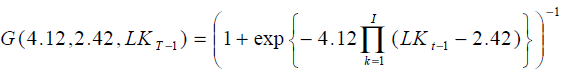(10)

In the first regime G=0 and in the second regime G=1 therefore, for first regime we have:

LCO2 (t) = 1.421LGDPP (t-2) + 0.89LEI (t-4) + 0.91LEI (t) + 0.014 LRPOP (t-3) + 0.003LRPOP (t) - 1.014LURBN (t-1) - 1.03LURBN (t-2)

In addition, for second regime we have:

LCO (t) = 2.41 + 1.45 LGDPP (t-1) - 0.85 LEI (t-2) + 0.76LEI (t) + 0.02 LRPOP (t-2) - 0.03 LRPOP (t) - 1.43 LURBN (t-1) - 1.12 LURBN (t-2)

The arguments in this paper, the effect of economic growth on environmental biology in consumption of energy in the new communities will provide. Comparing the situation in our country we reach points that are very important.

Conclusion

The goal of this paper was to test the existence of long run relationship economic growth on environmental biology consumption of energy in Iran. This objective was aid by the technique of Liew [13] approach to linear or non-linear model, which presents non-spurious estimates. Subsequently, our work provides fresh evidence on the long run relationship between economic growths on environmental biology consumption of energy in Iran. The results at relationship between economic growth on environmental biology consumption of energy studies of Alam and et. al. [7] and Ang [16] but our results are more robust.

Based on the results obtained can be stated that elasticity or sensitivity to carbon dioxide emissions per capita than positive per capita GDP, is significant and equal to 1.42. This issue shows that with increasing one percent in GDP per capita, the per capita carbon dioxide emissions and environmental pollution increases rate of 1.42 percent. In explaining this phenomenon mainly not taking advantage of new technologies with less pollution in the production of goods and services and also continuation and expansion activity some energy industry and the pollutants can outline the reasons being this coefficient. The findings theoretical foundations provided that to express economic growth causes increased environmental pollution, is both sides. Traction and sensitivity carbon dioxide emissions per capita than energy (Intensity Use of energy) Positive, Significant and equal to 0.89 the linear relationship and 0.85 The nonlinear relationship the increase one percent the intensity of energy use, the per capita carbon dioxide emissions increases rate of 0.89 percent. Efficient use of energy the price variations, low energy equipment technology, Also too much of some energy the more contaminant you can count on the main reason for the positive this coefficient is high. Theoretical research findings with also is consistent that Increased energy consumption causes increased environmental pollution. So, can be said carbon dioxide emissions per capita in the period studied than GDP per capita is elastic and sensitive and the relative increase in these variables increases more quickly.

References

1. Kuzents S.S. Amer. Econ. Rev. 1955, 45: 1–28.
2. Behbodi D., Barghi E. Quar. Eghtesade Meghdari, 2008, 5(4): 35-53.
3. Hasanzadeh A. J. Tazehaye Eghtesad, 2009, 7(126): 37-51.
4. Bagheri M. Quar. Ener. Econ. Stud. 2010, 7(27): 101-129.
5. Shim J.H. Cas. Stud. Sourh korea: Vniversity of Delaware, 2006.
6. Sadeghi H., Saadat R. J. Tahghighate Eghtesadi, 2004, 64: 163-180.
7. Alam S., Ambreen F., Muhammad B. J. Asi. Econ. 2007, 18: 825-837.
8. Grossman G.M., Krueger A.G. Nat. Bure. Econ. Res: NBER Work. Pap. 1991.
9. Shafik N., Bandhopadhyay S. Wor. Ban. Washin. D.C, 1992.
10. Panayotou T. Cent. Int. Develop. 2000.
11. Roca J., Padilla E., Farre M, Galletto V. Ecol. Econ. 2001, 39: 85-99.
12. Selden T.M., Song D. J. Env. Econ. Manag. 1994, 27: 147-162.
13. Liew V.K., Ahmad Z., Sie-Hoe L. Dep. Econ. Univ. Putra. Malaysia. 2002.
14. Meese R., Rogoff K. J. Int. Econ. 1983, 14(1): 3-24.
15. Dickey D., Fuller W.A. J. Amer. Statis. Assoc. 1979, 74: 427 – 431.
16. Ang T.B. Ener. Poli. 2007, 35: 4772- 4778.