Keywords
Non-zero ending inventory; Perishable goods; Selling price; Stock-dependent demand
Introduction
Deterministic inventory models usually consider the demand rate to be either constant or time-varying, but independent of level of inventory i.e. level of stock. However, it has been noted, especially in the retail market, that these inventory models are not suitable for representations of the reality of inventory control situation in the retail field. Levin et al. quoted that “large piles of goods attract more customers” this is termed as stock-dependent demand [1]. To incorporate this scenario into inventory models, a variety of stock-dependent demand models have been proposed. Baker and Urban established an Economic Order Quantity (EOQ) inventory model by specifying the stock-dependent demand as a power function with diminishing return of displayed stock level [2]. Urban extended the classical EOQ inventory model from zero ending inventories to non-zero ending inventory when the demand is dependent on the amount of displayed stocks [3]. Urban computed optimal order quantity when demand is stock-dependent [4]. Shah and Pandey presented an EOQ model where demand was dependent on stock displayed and advertisement frequency [5]. An EOQ model with delay in payments and stock dependent demand was given by Sarkar [6]. Sarkar and Sarkar developed better model for time-dependent deteriorating inventory when demand is stock dependent [7]. Shah et al. formulated an integrated inventory model with stock dependent demand. Shah and Shah developed an EOQ model for deteriorating items with imperfect quality and stock dependent demand under the effect of inflation [8,9]. Sarkar et al. presented a model for preservation of deteriorating seasonal products with stock-dependent demand [10]. Mishra and Shaikh formulated a two warehouse integrated inventory model for stock dependent demand rate with order size dependent trade credit [11]. Mishra et al. developed an EOQ model with price sensitive stock dependent demand with shortages. This implies that holding higher inventory level will probably make the retailer earn more profit by selling more items. Under this situation, the demand rate should depend on the level of inventory [12].
Recently, it is noted that customers are becoming more health conscious than before because of their continuously improving lifestyle. Hence, the demand for fresh items (e.g., vegetables, fruits, baked goods, bread, milk and seafood) has increased in recent years. In today’s market, determining price and order quantity jointly for retailers to better manage perishable products is recognized as an important way to increase profitability and maintain competitiveness in a supply chain. The traditional EOQ models assume that products can be stored indefinitely to meet future demand. However, many perishable products such as fruits, vegetables, medicines, and volatile liquids degrade or deteriorate continuously due to evaporation, spoilage, obsolescence or some other reasons. Most researchers modeled the effect of perishability in the past only from the retailer’s perspective as the on-hand stocks shrink due to damage, spoilage, dryness, vaporization, etc. Researchers rarely developed the effect of perishability into their models from the costumer’s perspective. In fact, freshness is one of the most critical criteria affecting customers purchasing decisions. Fujiwara and Perera took the effect of product freshness on consumer demand into consideration [13]. Subsequently, Sarker et al. studied the inventory policies for perishable products when the demand is negatively impacted by the age of the on-hand stocks [14]. Bai and Kendall then proposed an EOQ inventory model for perishable goods by extending the demand to be freshness and shelf-space dependent [15]. Many perishable goods (e.g., packed food, fruit and vegetable salads, donuts, milk, etc.) have only a few days of shelf life, and their demand rates gradually decline to zero as the expiration dates approach. By taking the expiration date into consideration, Wu et al. established the retailer’s optimal replenishment cycle time and ending stock level when the demand rate is a multivariate function of the product freshness and displayed stock level. Chen et al. further expanded the inventory model by Wu et al. to obtain the retailer’s optimal lot-size, shelf-space, and ending-stock by considering the shelf-space size as another decision variable [16,17]. Other recent research publications related to maximum lifetime span are studied in Sarker, Wang et al., and Wu et al. To better manage food near its expiry date at the retail stage, Aiello et al. studied the optimal time to withdraw the food from the shelf [18-20].
It has been noted that the demand of an item is affected by its price, consumer may opt for an alternative where he gets better deal. So in today’s competitive markets, determining price and order quantity jointly for retailers is recognized as an important way to increase profitability and maintain competitiveness in a supply chain. The demand rate is usually influenced by price of an item. Urban and Baker further generalized the demand rate as a multivariate function of price and displayed stocks level [21]. Teng and Chang expanded the EOQ inventory model with price and stock-dependent demand to an Economic Production Quantity (EPQ) inventory model for deteriorating items [22]. Feng et al. presented an EOQ model with demand as a multivariate function of price, stock and freshness of the product [23]. So the research in area of price and stock dependent demand is extensive.
This paper develops an EOQ model in which the demand of product is dependent on the freshness of item its selling price and displayed stock. Selling price crucially affects not only the demand rate but also the total profit. As a result, the selling price is considered as a decision variable in this paper. The objective of this study is to determine jointly the optimal unit price, cycle time and nonzero ending inventory that maximize the total profit of the retailer. The remainder of this paper includes notations and assumptions used in this paper, then the mathematical modelling is done by incorporating the demand as a multivariate function of unit selling price, displayed stocks and freshness of the item. Thereafter, numerical example is presented to validate the model. Sensitivity analysis for key parameters is done to observe their effect on decision variables. Lastly, we have described the conclusion of this paper with future research directions.
Notation and Assumptions
The proposed model uses the following notation and assumptions.
Notation
Cr Retailer’s unit purchase cost
hr Holding cost per annum
Ar Retailer’s ordering cost per order
δ Percentage discount in selling price for salvage value
m Maximum life time of item
I(t) Inventory level with retailer at time t.
Decision variables
E Ending inventory level in units E ≥ 0
S Retailer unit selling price, S > Cr
T Replenishment cycle time
Functions
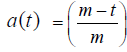 ; Age dependent freshness at time t, which is decreasing function of time lying between [0,1]
D(S,t) Demand rate depends on the freshness of the stock displayed and unit & selling price;, where α > 0 scale demand, stock dependent parameter and m is fixed life time of item.
π(E,S,T) Retailer total profit
The objective of the model is expressed as below:
Max π(E,S,T)
Subject to, S > Cr and E,S,T ≥= 0
Assumptions
1. Inventory system consists of single deteriorating item possessing fixed life time. At the beginning of the cycle inventory items are fully fresh (i.e. of freshness value 1) and their freshness decreases with time (i.e. depletes to zero by the end of their life span).
2. Demand of the product is dependent on the freshness of the stock displayed and its unit selling price. Here the standard assumption of zero ending inventory is given up as It might be beneficial to close out the sale at a nonzero ending inventory and have fresh stock for sale, because fresher items would attract more.
3. The nonzero ending inventory is sold out with attractive discount rate.
4. Replenishment is infinite, lead time is zero and shortages are not allowed.
Mathematical Model
In the proposed model, we consider a retailer dealing with a single item. The demand is dependent on freshness of the displayed stock and its selling price. It might be beneficial to close out sale at a lower rate, and keep on-hand fresh displayed stocks, because the demand is freshness and stock dependent. At the end of cycle time inventory level depletes to non-negative ending inventory i.e. E ≥ 0, which is sold for salvage value. The following differential equation represents the status of inventory during interval [0,T]:
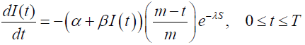 (1)
(1)
with I(0) = Q and I(T) = E. The solution of using I(T) = E is,
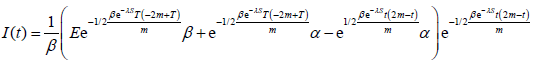 (2)
(2)
Using the other condition I(0) = Q and, we have
 (3)
(3)
The inventory holding cost is given by,
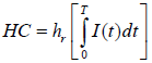 (4)
(4)
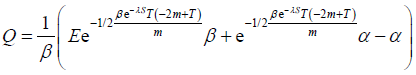
Therefor the total profit per unit time is given by,
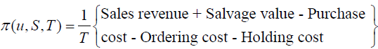 (5)
(5)
In this model total profit of the firm is to be maximized with respect to nonzero ending inventory (E), selling price (T) and cycle time (T).
Therefore, the optimization problem is,
Maximize,
Subject to, S > Cr and E,S,T ≥= 0
Next, we follow the following steps listed below to have an optimal solution.
Algorithm
Step 1: Assign numerical values to all the inventory parameters.
Step 2: Set 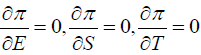 and solve simultaneously for u,S and T.
For the obtained solution check the concavity through graphs.
Numerical Examples
Example 1: Consider α = 1500, β=15%, λ= 0.22, m=0.2 year, Cr = $5 per unit, δ = 50%, $20 Ar = per order and $2 hr = inventory. The concavity of the given profit function is also shown in Figures 1-3.
Figure 1: Concavity of profit function for S=$10.37.
Figure 2: Concavity of profit function for T=0.0956 year.
Figure 3: Concavity of profit function for E=3.64 units.
Here the maximum profit is π = $407.26 for cycle time is S = $10.37 selling price S = $10.37 . The ordering quantity is E = 3.64 units with E = 3.64 as nonzero ending inventory. The concavity of the given profit function is also shown in Figures 1-3. Sensitivity analy sis
With the values of inventory parameters taken in example 1, sensitivity analysis of the optimal solution with respect to inventory parameters is done by changing one parameter at a time. The results obtained are shown in Table 1.
| Parameter |
Value |
E* |
S* |
T* |
Q* |
π |
| α |
1450 |
3.588 |
10.377 |
0.09734 |
14.489 |
386.776 |
| 1500 |
3.647 |
10.371 |
0.09566 |
14.806 |
407.26 |
| 1550 |
3.704 |
10.365 |
0.09406 |
15.118 |
427.863 |
| β |
0.12 |
3.653 |
10.373 |
0.09565 |
14.803 |
407.145 |
| 0.15 |
3.647 |
10.371 |
0.09566 |
14.806 |
407.26 |
| 0.18 |
3.641 |
10.369 |
0.09567 |
14.809 |
407.374 |
| λ |
0.2 |
1.341 |
10.335 |
0.08705 |
14.282 |
551.445 |
| 0.22 |
3.647 |
10.371 |
0.09566 |
14.806 |
407.26 |
| 0.24 |
5.305 |
10.411 |
0.10532 |
14.881 |
293.395 |
| m |
0.18 |
3.365 |
10.354 |
0.09114 |
13.84 |
386.386 |
| 0.2 |
3.647 |
10.371 |
0.09566 |
14.806 |
407.26 |
| 0.22 |
3.917 |
10.387 |
0.09989 |
15.715 |
425.113 |
| δ |
0.48 |
1.779 |
9.973 |
0.09592 |
13.98 |
413.042 |
| 0.5 |
3.647 |
10.371 |
0.09566 |
14.806 |
407.26 |
| 0.52 |
5.469 |
10.804 |
0.09574 |
15.623 |
397.152 |
| Ar |
4.5 |
1.34 |
9.35 |
0.09077 |
14.806 |
486.971 |
| 5 |
3.647 |
10.371 |
0.09566 |
14.806 |
407.26 |
| 5.5 |
5.151 |
11.395 |
0.10152 |
14.422 |
332.914 |
| Ar |
19 |
3.55 |
10.361 |
0.09317 |
14.532 |
417.852 |
| 20 |
3.647 |
10.371 |
0.09566 |
14.806 |
407.26 |
| 21 |
3.741 |
10.38 |
0.09809 |
15.069 |
396.937 |
| hr |
1.8 |
3.541 |
10.334 |
0.09594 |
14.814 |
408.982 |
| 2 |
3.647 |
10.371 |
0.09566 |
14.806 |
407.26 |
| 2.2 |
3.75 |
10.408 |
0.09538 |
14.796 |
405.526 |
Table 1: Numerical results.
The observations made from these calculations are: Increase in scale demand increases the order quantity, total profit and ending inventory; whereas the selling price and cycle time decreases (which implies higher demand shortens cycle time and increases profit). For increase in stock dependent parameter cycle time, ordering quantity and profit increases; whereas the selling price and ending inventory decreases. With increase in price efficiency of demand λ, ending inventory, selling price, cycle time, ordering quantity increase and total profit decreases.
Increase in maximum lifetime of item elevates all the decision variables, leading to more profit. Increase in percentage discount increases ending inventory, selling price, cycle time and order quantity resulting decrease in profit. Increase in purchase cost per unit increases the ending inventory, selling price and cycle time; which in result decreases order quantity and total profit. Increase in ordering cost hikes up all decision variables lowering the total profit. Lastly, increase in holding cost increases the ending inventory, selling price; whereas cycle time, order quantity and total profit decreases.
Numerical results in Table 1 demonstrates that the total profit is more sensitive to scale demand λ, price efficiency of demand λ, maximum lifetime of item m, discount rate and the purchase cost of item. Hence, the retailer needs to pay more attention to these parameters than others (Table 1).
Conclusion
In this paper, the objective is to determine optimal policies for retailer which maximizes his profit. The demand of an item is considered to be dependent on stock displayed, its selling price and the freshness of the items. The standard assumption of inventory level depleting to zero is relaxed here, instead it might be beneficial for the retailer to close out sale and stock up fresh items which boosts his demand. The retailer profit is maximized by considering cycle time, selling price and nonzero ending inventory decision variables Proposed model can be extended by allowing shortages, trade credit and investment in preservation technology. Model can be reviewed with stochastic demand also.
References
- Levin RI, Mclaughlin CP, Lamone RP, Kottas JF (1972) Productions/Operations Management Contemporary policy for managing operating systems. Macgraw-Hill, New York, USA.
- Baker RC, Urban TL (1988) A deterministic inventory system with an inventory level dependent demand rate. J Oper Res Soc 39: 823-831.
- Urban TL (1992) An inventory model with an inventory-level-dependent demand rate and relaxed terminal conditions. J Oper Res Soc 43: 721-724.
- Urban TL (2005) Inventory models with inventory level dependent demand: A Comprehensive review and unifying theory. Eur J Oper Res 164: 792-304.
- Shah NH, Pandey P (2009) Deteriorating inventory model when demand depends on advertisement and stock display. International J Operations Res 6: 33-44.
- Sarkar B (2012) An EOQ model with delay in payments and stock dependent demand in the presence of imperfect production. Appl Math Comput 218: 8295-8308.
- Sarkar B, Sarkar S (2013) An improved inventory model with partial backlogging, time varying deterioration and stock-dependent demand. Econ Model 30: 924-932.
- Shah NH, Shah AD (2014) Optimal cycle time and preservation technology investment for deteriorating items with price-sensitive stock-dependent demand under inflation. J Phys Conf Ser 495: 012017.
- Shah NH, Patel DG, Shah DB (2014) Optimal integrated inventory policy for stock-dependent demand when trade credit is linked to order quantity. Revista Investigación Operacional 35: 130-140.
- Sarkar S, Mandal B, Sarkar B (2016) Preservation of deteriorating seasonal products with stock-dependent consumption rate and shortages. J Ind Manag Optim 13: 187-206.
- Mishra P, Shaikh A (2017) Optimal ordering policy for an integrated inventory model with stock dependent demand and order linked trade credits for twin ware house system. Uncertain Supply Chain Management 5: 169-186.
- Mishra U, Cárdenas-Barrón LE, Tiwari S, Shaikh AA, Treviño-Garza G (2017) An inventory model under price and stock dependent demand for controllable deterioration rate with shortages and preservation technology investment. Ann Oper Res 254: 165-190.
- Fujiwara O, Perera ULJSR (1993) EOQ models for continuously deteriorating products using linear and exponential penalty costs. Eur J Oper Res 70: 104-114.
- Sarker BR, Mukherjee S, Balan CV (1997) An order-level lot size inventory model with inventory-level dependent demand and deterioration. Int J Prod Econ 48: 227-236.
- Bai R, Kendall G (2008) A model for fresh produce shelf-space allocation and inventory management with freshness-condition-dependent demand. Informs J Comput 20: 78-85.
- Wu J, Chang CT, Cheng MC, Teng JT, Al-Khateeb FB (2016) Inventory management for fresh produce when the time-varying demand depends on product freshness, stock level and expiration date. International J Systems Science: Operations & Logistics: 3: 138-147.
- Chen SC, Min J, Teng JT, Li F (2016) Inventory and shelf-space management for fresh produce with freshness-and-stock dependent demand and expiration date. J Oper Res Soc 67: 884-896.
- Wang WC, Teng JT, Lou KR (2014) Seller’s optimal credit period and cycle time in a supply chain for deteriorating items with maximum lifetime. Eur J Oper Res 232: 315-321.
- Wu J, Ouyang LY, Cárdenas-Barrón LE, Goyal SK (2014) Optimal credit period and lot size for deteriorating items with expiration dates under two-level trade credit financing. Eur J Oper Res 237: 898-908.
- Aiello G, Enea M, Muriana C (2014) Economic benefits from food recovery at the retail stage: An application to Italian food chains. Waste Manag34: 1306-1316.
- Urban TL, Baker RC (1997) Optimal ordering and pricing policies in a single-period environment with multivariate demand and markdowns. Eur J Oper Res 103: 573-583.
- Teng JT, Chang CT (2005) Economic production quantity models for deteriorating items with price- and stock-dependent demand. Comput Oper Res 32: 297-308.
- Feng L, Chan Y, Cárdenas-Barrón LE (2017) Pricing and lot-sizing polices for perishable goods when the demand depends on selling price, displayed stocks, and expiration date. Int J Prod Econ 185: 11-20.