Key words
Industry sector Growth, monetary Policy, unit root test, autoregressive distributed
lag (ARDL).
Introduction
In the literature, macroeconomists have established the theoretical relationship between real
output and monetary policy measures. To Keynesians, a discretionary change in money supply
permanently influences real output by lowering the rate of interest and through the marginal
efficiency of capital, stimulate investment and output growth [2,3]. In contrast to Keynesian
policy prescription, McKinnon [4] and Shaw [5] in advocating the financial liberalization
hypothesis argued that a market force induced higher interest rate, would enhance more
investment by channeling saving to productive investment and stimulate real output growth.
Based on these theoretical propositions, empirical questions have been raised on whether this
consensus views on the effect of monetary policy on the real output holds for the different
sectors of the economy. Existing studies have shown that the effects of monetary policy on
sectors output varies and such variation might arise because of the relative strength of a
particular channel of monetary of transmission mechanism on some sectors than for sectors [6].
Also, the possibility of a differential response between sect oral output and aggregate output to
monetary policy measures has been investigated by Granley and Salmon [7] for other countries.
In many regards, the recent history of monetary economics can be understood as exploring
different elements of the monetary authority’s constrained maximization program. In the early
1970s debate focused on the “instrument choice” question, and whether monetary policy should
target the interest rate or money supply. Poole [8] examined this question within the context of
the neo-Keynesian ISLM model. Sargent and Wallace [9] examined it using a new classical
rational expectations (RE) model. Post-Keynesians, with their theory of endogenous money
supply [10] have criticized this debate arguing that money supply targeting is infeasible because
the money supply is determined by bank lending. That means the monetary authority can only
target the interest rate.
The mid-1970s and early 1980s saw a dramatic change in the framing of the optimal monetary
policy problem. Lucas [11] adopted a classical macroeconomic framework with rational
expectations (RE), and argued that “fooling” workers about inflation explains why output and
employment respond positively to inflation. His work triggered a two-fold shift. First, and most
importantly, there was a shift from using Keynesian economics to describe the structure of the
economy to using classical macroeconomics. Second, RE shifted attention to issues of the
distribution of information about inflation, learning and agents’ responses to monetary policy
[11]. Thus, the effectiveness and impact of policy could change as agents learned and responded.
Concern with learning and response then directed attention toward time and game theoretic
considerations. Kydland and Prescott [12] introduced the time-consistency problem for monetary
policy, while Barro and Gordon [13] introduced gaming between the monetary and economic
agents. These concerns in turn triggered interest in issues of policy credibility, giving rise to the
“rules vs. discretion” policy literature [14]. Additionally, these models tacitly smuggled in the
assumption that the monetary authority’s social welfare function was different from the public’s
welfare function, which contrasts with the Keynesian literature that assumed a benevolent policy
maker [15].
Monetary Policy in Islamic Republic of Iran
After the Islamic revolution in Iran, at 1979, there were comprehensive attempts by government
to use Islamic rules and regulations in all aspects of society and economic and banking system of
the country was one these aspects. Finally at 1983 economic experts and Shariah scholars
provided the Interest Free Banking System Bill to the parliament that used Islamic contracts as
instruments for attracting and allocating money in the banking system. After approving process
by parliament, and Guardian Council, which contains 6 lawyers and 6 Islamic jurists who
monitor all parliament approvals not to be against Islamic rules, from the 1984, the whole
economic and banking system of country changed to Islamic one. Unlike some Islamic countries
which have both Islamic and non-Islamic banking system, there is not any bank in Iran that
works according to interest rate system. From the beginning of the Islamic banking system, the
central bank of Iran did its best to use monetary policy instruments which have no contradiction to Islamic rules and at the same time bring macroeconomic stability and growth to the country.
We can see that Central Bank of Iran does not restrict itself only to monetary aggregate
instrument of monetary policy and uses extensively from profit rate instrument like Musharakah
certificates. Here, we explain the instruments that central bank currently uses to execute
monetary policy1.
Monetary Policy Instruments in Iran2
In implementing monetary policy, the Central Bank can directly resort to its regulating power or
affect money market conditions indirectly as issuer of high-powered money (notes and coins in
circulation and deposits held with Central Bank). On this basis, two different monetary policy
instruments are being utilized: direct instruments (with no reliance on market conditions) and
indirect instruments (market-oriented).
Direct Instruments
With the implementation of Usury-free Banking Law and the introduction of contracts with fixed
return and partnership contracts, the regulations pertaining to determination of profit rate or
expected rate of return on banking facilities and the minimum and maximum profit rate or
expected rate of return, as is stipulated in the by-law of the Usury free Banking Law, are
determined by the Money and Credit Council (MCC). Moreover, the Central Bank of Iran (CBI)
can intervene in determining these rates both for investment projects or partnership and for other
facilities extended by banks. According to Article 14 of the Monetary and Banking Law of Iran,
the CBI can intervene in and supervise monetary and banking affairs through limiting banks,
specifying the mechanisms for use of funds and determining the ceiling of loans and credits in
each sector.
Indirect Instruments
Reserve Requirement Ratio (RRR) is one of the CBI’s indirect instruments of monetary policy.
Banks are obliged to deposit part of their liabilities in the form of deposit with the CBI. Through
increasing/decreasing this ratio, the CBI contracts/expands the broad money. According to
Article 14 of the Monetary and Banking Law of Iran, the CBI is authorized to determine RRR
within 10 to 30 percent depending on banks’ liabilities’ composition and field of activity.
Appropriate implementation of monetary policies by the CBI is done through open market
operations, which provide the required flexibility in liquidity management and intervention in the
money market. Following the implementation of the Usury free Banking Law, tailoring
appropriate Sharia-based instruments for the development of open market operations in the
context of liquidity management and affecting money and capital market became a necessity.
Utilization of bonds, owing to its fixed interest rate nature, is prohibited according to Islamic
Sharia; however, utilization of participation papers and investors’ partnership in economic
activities and payment of profit is encouraged. According to the 3rd FYDP3 Law, the CBI was
authorized to issue participation papers through the MCC approval. However, based on the 4th FYDP Law, issuance of Participation Papers by the CBI is authorized upon the approval of the
Parliament. By using this instrument, the CBI could affect broad money (M2) through monetary
base, thereby controlling the rate of inflation. One of the bold measures taken for the efficient
utilization of indirect monetary instruments in the framework of the Usury-free Banking Law is
to allow banks to open a special deposit account with the CBI. Regulation on ODA was
approved by the MCC at the end of 1998-99. The main objective of this plan was the adoption of
appropriate monetary policies to control liquidity through absorption of banks’ excess resources.
The CBI pays profit to these deposits on the basis of specific rules.
The present research explores from macro perspective an alternative way in which the industry
sector growth could be explored employing time series data. Following Bernanke and Blinder
[16], the real output is inversely related to the interest rate but it is shifted by monetary policy, R,
and by credit shock that affected either the loans demand or supply functions [17]. For that
purpose, we use the bounds testing (or ARDL) approach to co-integration proposed by Pesaran et
al. [1] to test the effects of monetary Policy on industry sector growth in Iran using data over the
period 1961–2007. The ARDL approach to co-integration has some econometric advantages
which are outlined briefly in the following section. Finally, we apply it taking as a benchmark
Bernanke and Blinder [16] study in order to sort out whether the results reported there reflect a
spurious correlation or a genuine relationship between on industry sector growth and the
variables in question. This contributes to a new methodology in the on industry sector growth
literature. Next section starts with discussing the model and the methodology. Then in Section 3
we describe the empirical results of unit root tests, the F test, ARDL co-integration analysis,
Diagnostic and stability tests and Dynamic forecasts for dependent variable and Section 4
summarizes the results and conclusions.
Materials and Methods
The model
Following the practice in the literature, the loan rate that cleared the loan market can be stated:
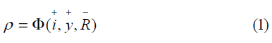
Equation (1) showed that the interest rate on loans was positively related to interest rate on bonds
and income, but inversely related to bank reserves. To solve for the aggregate demand curve;
Bernanke and Blinder [16] used the following generic IS curve:
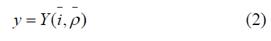
And then by substituting equation (1) into (2), we have:
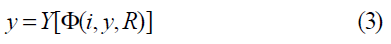
As expressed by Bernanke and Blinder [16] the real output is inversely related to the interest rate
but it is shifted by monetary policy, R, and by credit shock that affected either the loans demand or supply functions [17]. By expressing equation (3) in more explicit forms and accommodating
other relevant variables in the model, equation (3) can be expressed as a simple linear equation
model is summarized as:

Where: Y= real output, INT= interest rate, EX= exchange rate, PSC = credit to the private
sector, ASP = all share price index, CPI = consumer price index
Equation (4) was the baseline model for the analysis of the effects of monetary policy on each of
the sect oral outputs. The following modified model in logarithm form is used to examine the
monetary policies in industry sector in Iran. The logarithm equation corresponding to Eq. (4) and
breakdown of the factors industry sector gives:

Where YI is real output in industry sector and PSCI is credit to the private sector in industry. Our
empirical analysis in Section 3 is based on estimating directly long-run and short-run variants of
Eq. (5). All the data in this study are obtained from Central Bank of Iran (2004)1 during the
period 1961-2007.
The methodology
Recent advances in econometric literature dictate that the long run relation in Eq. (5) should
incorporate the short-run dynamic adjustment process. It is possible to achieve this aim by
expressing Eq. (5) in an error correction model as suggested by Engle and Granger [18]. Then,
the equation becomes as follows:
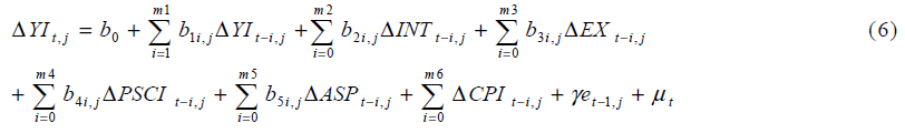
Where Δ represents change, mi is the number of lags, γ is the speed of adjustment parameter and
εt−1 is the one period lagged error correction term, which is estimated from the residuals of Eq.
(5). The Engle–Granger [18] method requires all variables in Eq. (5) are integrated of order one,
I (1) and the error term is integrated order of zero, I (0) for establishing a co-integration
relationship. If some variables in Eq. (5) are non-stationary we may use a new co-integration
method proposed by Pesaran et al. [1]. This approach is also known as Auto Regressive
Distributed Lag (ARDL) that combines Engle and Granger [18] two steps into one by replacing
εt−1 in Eq. (6) with its equivalent from Eq. (5). εt−1 is substituted by linear combination of the
lagged variables as in Eq. (7).
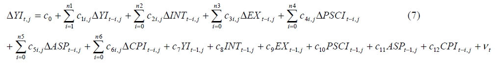
To obtain Eq. (7), one has to solve Eq. (5) for εt and lag the solution equation by one period.
Then this solution is substituted for εt−1 in Eq. (6) to arrive at Eq. (7). Eq. (7) is a representation
of the ARDL approach to co-integration. Pesaran et al. [1] co-integration approach, also known
as bounds testing, has some methodological advantages in comparison to other single cointegration
procedures. Reasons for the ARDL are: i) endogenous problems and inability to test
hypotheses on the estimated coefficients in the long-run associated with the Engle and Granger
[18] method are avoided; ii) the long and short-run coefficients of the model in question are
estimated simultaneously; iii) the ARDL approach to testing for the existence of a long-run
relationship between the variables in levels is applicable irrespective of whether the underlying
regresses are purely stationary I(0), purely non-stationary I(1), or mutually co-integrated, and iv)
the small sample properties of the bounds testing approach are far superior to that of multivariate
co-integration, as argued in Narayan [19]. The procedure is no longer valid in presence of I (2)
series (integrated of order 2). Given that Pesaran et al. [1] co-integration approach is a relatively
recent development in the econometric time series literature, a brief outline of this procedure is
presented as follows. The ARDL approach involves two steps for estimating the long-run
relationship. The bound testing procedure is based on F-statistics and is the first step of the
ARDL co-integration method. Accordingly, a joint significance test that implies no cointegration
under the null hypothesis, (H0: c4=c5=c6=0), against the alternative hypothesis, (H1:
at least one c4 to c6≠0) should be performed for Eq. (7). The F test used for this procedure has a
non-standard distribution. Thus, Pesaran et al. [1] computed two sets of asymptotic critical
values for testing co-integration for a given significance level with and without a time trend. One
set assumes that all variables are I (0) and the other set assumes they are all I (1). If the computed
F-statistic exceeds the upper bound critical value, then the null hypothesis of no co-integration
can be rejected. Conversely, if the F-statistic falls below the lower bound critical value, the null
hypothesis cannot be rejected. Lastly, if the F-statistic falls between these two sets of critical
values, the result is inconclusive. The short-run effects between the dependent and independent
variables are inferred by the size of coefficients of the differenced variables in Eq. (7). The longrun
effect is measured by the estimates of lagged explanatory variables that are normalized on
estimate of c4. Once a long-run relationship has been established, Eq. (7) is estimated using an
appropriate lag selection criterion. At the second step of the ARDL co-integration procedure, it is
also possible to obtain the ARDL representation of the Error Correction Model (ECM). To
estimate the speed with which the dependent variable adjusts to independent variables within the
bounds testing approach, following Pesaran et al. [1] the lagged level variables in Eq. (7) are
replaced by ECt−1 as in Eq. (8):
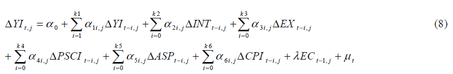
A negative and statistically significant estimation of λ not only represents the speed of
adjustment but also provides an alternative means of supporting co-integration between the
variables.
Structural stability tests Cumulative Sum (CUSUM) and Cumulative Sum of Square
(CUSUMSQ)
There are two statistical methods to test the structural stability of the restricted autoregressive
models. These are the cumulative sum and the cumulative sum of squares tests of recursive
residuals, which can be shown graphically in the Microfit displays two straight lines that
represent the 5 per cent critical bounds where the null hypothesis of having stable parameters for
each of the five observed variables is rejected if any of the straight lines is significantly crossed.
Otherwise, if the plot generally remains within those two straight lines, the null hypothesis is not
rejected. The cumulative sum test helps to show if the coefficient of regression are changing
systematically, whereas the cumulative sum of squares test is helpful in showing if the regression
coefficients are changing suddenly. These tests have been proposed by Brown et al. [20]. Its
foundation is based on that initially, a regression equation including the variable desired is
estimated using of estimated to be at least observations. Then, one observation is added to the
observations of previous equation and next estimation is performed and in this same way, it is
added to the observations a unit. In this way, after the estimation of each step, one coefficient is
obtained for any of the variables which finally is concluded a time series of variables
coefficients. These tests presents Cumulative sum (CUSUM) and cumulative sum of Square
(CUSUMSQ) diagrams between two straight lines (the bounds of the 95 percent).If the diagram
presented be within the boundaries, zero hypothesis is accepted which is based on lack of
structural break and if the diagram go out of the boundaries (it means that if dealt to them), zero
hypothesis is rejected which is based on lack of structural break and the presence of structural
break is accepted [21]. CUSUM statistics is useful to find systematic changes in long term
coefficients of regression and CUSUMSQ statistics is helpful when deviation from regression
coefficients stability is randomized and occasional (short term).
Results and Discussion
Unit Root Test
We use the Augmented Dickey-Fuller [22] t-statistic when to difference time series data to make
it stationary. Here are the various cases of the test equation:
A. When the time series is flat (i.e. doesn’t have a trend) and potentially slow-turning around
zero, we use the following test equation:

Where the number of augmenting lags (p) is determined by minimizing the Schwartz Bayesian
information criterion or minimizing the Akaike information criterion or lags are dropped until
the last lag is statistically significant. Mifrofit allows all of these options to choose from. This
test equation does not have an intercept term or a time trend. Unfortunately, the Dickey-Fuller tstatistic
does not follow a standard t-distribution as the sampling distribution of this test statistic
is skewed to the left with a long, left-hand-tail. Microfit will give us the correct critical values for the test, however. Notice that the test is left-tailed. The null hypothesis of the Augmented
Dickey-Fuller t-test is:
H0: θ = 0 (i.e. the data needs to be differenced to make it stationary)
Versus the alternative hypothesis of:
H1: θ < 0 (i.e. the data is stationary and doesn’t need to be differenced)
B. When the time series is flat and potentially slow-turning around a non-zero value, we use the
following test equation:

Notice that this equation has an intercept term in it but no time trend. Again, the number of
augmenting lags (p) is determined by minimizing the Schwartz Bayesian information criterion or
minimizing the Akaike information criterion or lags are dropped until the last lag is statistically
significant. Microfit allows all of these options to choose from. We then use the t-statistic on the
θ coefficient to test whether we need to difference the data to make it stationary or not. Notice
the test is left-tailed. The null hypothesis of the Augmented Dickey-Fuller [22] t-test is:
H0: θ = 0 (i.e. the data needs to be differenced to make it stationary)
Versus the alternative hypothesis of:
H1: θ < 0 (i.e. the data is stationary and doesn’t need to be differenced)
C. When the time series has a trend in it (either up or down) and is potentially slow-turning
around a trend line we would draw through the data, use the following test equation:

Notice that this equation has an intercept term and a time trend. Again, the number of
augmenting lags (p) is determined by minimizing the Schwartz Bayesian information criterion or
minimizing the Akaike information criterion or lags are dropped until the last lag is statistically
significant. Microfit allows all of these options for us to choose from. We then use the t-statistic
on the θ coefficient to test whether we need to difference the data to make it stationary or we
need to put a time trend in our regression model to correct for the variables deterministic trend.
Notice the test is left-tailed. The null hypothesis of the Augmented Dickey-Fuller [22] t-test is:
H0: θ = 0 (i.e. the data needs to be differenced to make it stationary)
Versus the alternative hypothesis of:
H1: θ < 0 (i.e. the data is trend stationary and needs to be analyzed by
means of using a time Trend in the regression model instead of differencing the data)
The results reported in Table 1 show that null hypothesis of ADF unit root is accepted in case of
LYI, LEX, LCPI and LPSCI variables but rejected in first difference at 1% level of significance.
This unit root test indicate that LYI, LEX, LCPI and LPSCI variables considered in the present
study are difference stationary I (1) while LINT and LASP variables are level stationary I(0) as
per ADF test. On the basis of this test, it has been inferred that LYI, LEX, LCPI and LPSCI
variables are integrated of order one I (1), while LINT and LASP variables are integrated of order
zero I (0). Under these circumstances and especially when we are faced with mix results,
applying the ARDL model is the efficient way of the determining the long-run relationship
among the variable under investigation. Therefore, we will apply this methodology in the section
3.3.
Table 1: Results of unit root by ADF test
ARDL co-integration analysis for agricultural value added with oil shocks as Structural
Breaks: The estimated coefficients of the long-run relationship and Error Correction Mode
(ECM) are displayed in Table 2,3. The significance of the Error Correction Term and F-statistics,
in Table 2, indicates causal and long term relation among the variables in Iran.
Table 2: Estimated long-run coefficients ARDL
Table 3: Estimated Error Correction Model
As we see in Table 3, ECM version of this model show that the error correction coefficient
which determined speed of adjustment, had expected and significant negative sign. Bannerjee et
al. [24] holds that a highly significant error correction term is further proof of the existence of a
stable long-term relationship. The results indicated that deviation from the long-term in
inequality was corrected by approximately 32 percent over the following year or each year. This means that the adjustment takes place relatively quickly, i.e. the speed of adjustment is relatively
high. Also, analyzing the stability of the long-run coefficients together with the short run
dynamics, the cumulative sum (CUSUM) and the cumulative sum of squares (CUSUMSQ) are
applied. According to Pesaran and Shin [25] the stability of the estimated coefficient of the error
correction model should also be empirically investigated. A graphical representation of CUSUM
and CUSUMSQ are shown in Figure 1.
Figure 1. Plots of CUSUM and CUSUMQ statistics for coefficients stability tests
Following Bahmani-Oskooee [21] the null hypothesis (i.e. that the regression equation is
correctly specified) cannot be rejected if the plot of these statistics remains within the critical
bounds of the 5% significance level. As it is clear from Figure 1, the plots of both the CUSUM and
the CUSUMSQ are within the boundaries and hence these statistics confirm the stability of the
long run coefficients of regressors which affect the inequality in the country. The stability of
selected ARDL model specification is evaluated using the cumulative sum (CUSUM) and the
cumulative sum of squares (CUSUMSQ) of the recursive residual test for the structural stability
(see Brown et al., [20]). The model appears stable and correctly specified given that neither the
CUSUM nor the CUSUMSQ test statistics exceed the bounds of the 5 percent level of
significance.
Conclusion
Expansionary monetary policy implemented can be affect real economic sector noticeably by
reduction in the legal deposit rates or increase in the banks debt to the Central Bank and can be
positive effects by increase in the production and employment level and increase in the
components of total demand and consequently improvements in public welfare. In this pattern,
exchange policies implemented by increase in the nominal exchange rate causes to decrease
imports and gross domestic product (GDP). Contrary to expectations, this policy affects on non
oil export and increase in the production noticeably. The goal of this paper was to test the
existence of long run relationship determinants of monetary policies industry sector in Iran. This
objective was aided by the technique of Pesaran et al. [21] approach to co-integration which
presents non-spurious estimates. Subsequently, our work provides fresh evidence on the long run
relationship between monetary policies industry sector in Iran. Results of this study represent
Volume of monetary and exchange policies effectiveness in Iran’s economy. This study showed
that output growth in the industry can also be enhanced through successful management of the domestic credit through moderate reduction in the cost of borrowing in the financial market.
More so, given the significant contribution of domestic credit in influencing the output growth of
industry sector, there is the need for monetary authority to reduce the extent of unproductive
credit directed to the public authority. Greater proportion of the aggregate domestic credit should
be directed to the private sector at a competitive rate with strict guidelines and monitoring. This
guidelines and supervision would prevent diversion of the credits to unproductive usage. Prudent
use of the credit would promote investment and consequently output growth across sector of the
economy.
1These Instruments are introduced in the website of Central Bank of Iran: www.cbi.ir
2Central Bank of Iran: www.cbi.ir
3Pre-revolution economic plans in Iran include: third plan during 1963-1967, fourth plan during 1968-1972, fifth plan during
1973-1977 and economic plans during war and Islamic revolution during 1978 through 1988 and also economic, social and
cultural development plans of Islamic republic of Iran including first plan during 1989-1993, second plan during 1994-1998,
third plan during 1999-2004 and fourth plan during 2005-2009.
References
- Pesaran, H. M., Shin, Y., Smith J. R. J. Appl. Econ., 2001, 16, 289–326.
- Molho, L. E. IMF Staff Paper, 1986, 83(1), 90-116.
- Athukorala, P. C. Oxford Development studies, 1998, 26(2), 153-169.
- McKinnon, R. Brook lings institutions, 1973.
- Shaw, E. Oxford University Press, 1973.
- Gruen, D. Sheutrim, G. Proc. Conf. Sidney: RBA, 1994, 309- 363.
- Granley, J., Salmon, C. Working paper No. 68. Bank of England. 1997.
- Poole, W., Quarterly J. Econ, 1970, 84: 197 - 216.
- Sargent, T.J., Wallace, N. Journal Polit. Econ, 1975, 83: 241-54.
- Moore, B.J., Horizontalists, Verticalists. Cambridge University Press, 1988.
- Lucas, R.E., Journal of Monetary Economics, 1976, 2:19-46.
- Kydland, F.E., Prescott, E.C. Journal of Political Economy, 1977, 85: 473 - 92.
- Barro, R.J. Gordon, D.B. Journal of Political Economy, 1983, 91:589 – 610.
- Taylor, J.B. Carnegie – Rochester Conference Series on Public Policy, 1993, 39: 195-214.
- Palley, T.I. Negatively Sloped, Vertical, and Backward-Bending Phillips Curves, manuscript, Washington DC, 2006.
- Bernanke, B. S., Blinder, S. A. American Economic Review, 78, Papers and Proceedings of the 100th Annual Meeting of the American Economics Association, 1988, 435-39.
- Azali, M. University Putra Malaysia Press. UPM Serdang. 2003.
- Engle, R. F., Granger, W. J. Econometrica, 1987, 55, 251-276.
- Narayan, P. K. App. Econ. 2005, 37:1979–1990.
- Brown, R. l., Durbin, J., Evans, J. M. J. Royal Statis. Soc. 1975, 37:141-192.
- Bahmani-Oskooee, M. Japan and World Economy, 2001, 13:455-461.
- Dickey, D., Fuller, W. A. J. American Statis. Association. 1979, 74:427 – 431.
- Fuller, W. A. Introduction to Statistical Time Series. New York, Wiley, 1976.
- Banerjee, A., Lumsdaine, R. L., Stock, J. H. J. Bus. Econ. Statistics, 1992, 10:271-287.
- Pesaran, H., Shin, Y. The Ragnar Frisch Centennial Symposium (Cambridge: Cambridge University Press), 1999.
- Kankal, S. B., Gaikwad, R.W. Advances in Applied Science Research, 2011, 2 (1), 63.
- Elinge, C. M., Itodo, A. U., Peni, I. J., Birnin-Yauri, U. A., Mbongo, A. N. Advances in Applied Science Research, 2011, 2 (4), 279.
- Ameh, E. G., Akpah, F. A. Advances in Applied Science Research, 2011, 2 (1), 33.
- Ogbonna, O., Jimoh, W. L., Awagu, E. F., Bamishaiye, E. I. Advances in Applied Science Research, 2011, 2 (2), 62.
- Yadav, S. S., Kumar, R. Advances in Applied Science Research, 2011, 2 (2), 197.
- Sen, I., Shandil, A., Shrivastava, V. S. Advances in Applied Science Research, 2011, 2 (2), 161.
- Levine, D. M., Sulkin, S. D. J. Exp. Mar. Biol. Eco. 1984, 81: 211-223.
- Gupta N., Jain U. K. Der Pharmacia Sinica 2011 2(1):256:262.