Keywords
GGE biplot; Multi-environment trials; Bayesian
approach
Introduction
Multi-environment trials (MET) are used to identify superior
crop genotypes for a target environment in plant breeding
programs [1,2]. Selecting the best genotypes, with stable and
high yield across a number of environments presents statistical
issues in the presence of significant genotype x environment interaction (GEI) due to changes in the magnitude of the
genotypic response across the environments [3]. GGE biplot has
been shown to be very useful for analyzing MET datasets and
identifying adaptable genotypes with high yield performance in
several studies [4-6]. The GGE biplot analysis exhibits the
aspects of genotype stability and adaptability, when a high
proportion of the sum of squares of G+GEI could be retained in
first two principal components [7]. The polygon view of the
biplot is the sound way to visualize the interaction patterns
between genotypes and environments [8]. Yan and Kang (2003)
have shown the presence or absence of crossover GE interaction
which is helpful in identifying different mega environments.
Recently, the extensive usefulness of GGE-biplot has been
elucidated for analyzing data from multi-environment trials in
wheat [9]. These aspects make GGE biplot a most
comprehensive tool in plant breeding. GGE biplot is for: 1)
carrying out mega-environment analysis (see example, [10-12]:
2) genotypes evaluation (the mean performance and stability)
and 3) environments’ evaluation (the power to discriminate
among genotypes in target environment). A two-way table of GE
data may be analyzed through the joint use of analysis of
variance (ANOVA) and singular value decomposition (SVD) in
term of principal component analysis (PCA) [13].
In an ongoing crop improvement program, priors information
is available for distribution of variance components, for example,
for genotypes and genotype x environment integration. These
can be used to improve the results on the predication of GE
means. The commonly used frequentist approaches also not
make use of such information. The analysis of multienvironment
trials with a view to estimate genotypes stability
can be carried out using a Bayesian approach. Edwards and [14]
modeled heterogeneity using exponential of an additive model
followed by assigning suitable priors to the variance components
of the effects terms of the model. Crossa et al. have studied
some practical and theoretical aspect of Bayesian stability in the
context of additive main effects and multiplicative interaction
(AMMI) and posterior means for genotype × environment
interaction component using Gibbs sampler and applied to data
on maize [15]. Applications of the Bayesian approach to the
AMMI model and GGE have been presented by Josse et al. [16] and da Silva et al. [17]. Using Bayesian analysis, Omer et al.
conducted a similar study on genotype × environment
interactions and the GGE-biplot assessment of balanced
classifications with missing values [18]. Bayesian analysis of GGE
biplot models and its implications for the interpretation of the
biplots have been discussed in de Oliveira et al. [19]. The
purpose of this study is to compare Bayesian and frequentist
approaches for GGE biplot of sorghum genotypes yields in six
environments in Sudan. The first section presents a frequentist
approach, the commonly used GGE biplots. The second section
is Bayesian GGE biplot analysis obtained from posterior
estimates of genotype × environment interaction of predicted
means of grain yield.
Materials and Methods
Experimental data set
Eighteen genotypes of sorghum were evaluated in
randomized complete block design (RCBD) during three growing
seasons, 2009/10 to 2011/12, at two different locations (North
Gedarif and South Gedarif) in Sudan. Data on grain yield in kg/ha
was recorded for analysis.
Statistical analysis
Analysis of variance (ANOVA) and REML methods were
applied on the combined data using Genstat software [20] to
obtain the frequentist estimates of variance components and
predicted means while R2WinBUGS was used to obtain posterior
means under Bayesian approach. GGE biplot graphs were drawn
based on predicted means of under frequentist and Bayesian
approach. Therefore, the Bayesian posterior means of GE two
ways table based on priors for the SDCs, priors were obtained by
using data on sorghum yield (kg ha-1) from three similar
experiments conducted to evaluate 18 genotypes in RCBDs with
four replications during 2006/07- 2008/09 at Rahd station in
Sudan. A priors information and the WinBUGS and R codes are
available [21], the number of iterations was set at one 50,000,
the number of chains was set at three, and the last 5,000
simulated values of the parameters were taken for evaluating
the posterior distributions.
The Bayesian approach uses prior information which was
considered in terms of distributions for variance or standard
deviation components for effects of blocks within environments,
genotypes, environments and GEI and experimental error variances σe2, assumed to be homogeneous across
environments. The a priori distributions of the variance
components in terms of the scale parameters, in the GEI model
in the application were taken from past data for half-normal
distributions. The prior of half- normal distribution was used for
the various standard deviation components of the data model.
Using the best a priori distributions, the a posteriori expected
values of predicted GE means were obtained (details are aimed
for presentation in a separate publication and are not included
here). Details of the deviance information criterion (DIC), a
Bayesian counterpart of the Akaike information criterion (AIC) for model selection, and selection of the best priors data see
[22,23].
The Bi-plots model
Yan and Kang (2003) observed phenotypic variation (P) of
genotypes across environments is made up of environment
variation (E), genotype variation (G) and genotype-byenvironment
(GE) interaction variation Yan [24,25]. This can be
written as P-E=G+GE, usually E is the dominant source of
variation separate for genotype, so environmental means are
removed and analysis concentrates on the genotype variation
and genotype-by-environment interaction [26]. The sum of
these two terms can be approximated as first two principal
components to obtain GGE bi-plot using Genstat software. The
basic model for a GGE bi-plot is given as
Yij=μ+bj +αi+dij (1)
Where Yij=the estimated yield of genotype i in environment j,
μ=the grand mean of all observations, αi=the main effect of
genotype i, bj=the main effect of environment j and dij=the
interaction between genotype i and environment j. Instead of
trying to separate G and GEI, a GGE biplot model accounts G and
GEI together and expresses their joint contribution G+GEI into
two multiplicative terms [27]. Thus, the GGE bi-plot model can
be rewritten as
Yij=μ+ bj+γ1Pi1δj1+γ2Pi2δj2+εij (2)
where γ1 and γ2 are the singular values (SV) for the first and
second principal component (PC1 and PC2), respectively, Pi1 and
Pi2 are elements of eigenvectors of genotype i for PC1 and PC2,
respectively, δj1 and δj2 are elements of eigen vectors of
environment j for PCl and PC2, respectively, εij is the residual
associated with genotype i in environment j. PC1 and PC2
eigenvectors cannot be plotted to uniquely construct a
meaningful bi-plot before the singular values are partitioned
into the genotype and environment eigenvectors. Singular-value
partitioning is implemented by,
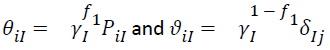 (3)
(3)
Where, I=1,2 and f1 is the partition factor for PC1.
Theoretically, f1 can be a value between 0 and 1, f1=1 is most
commonly used and is interpreted as environment focused. To
generate the GGE bi-plot, the equation [1] is presented as:
Yij=μ+ bj+θi1ϑ1j+θi2ϑ2j+εij (4)
In a bi-plot, genotype i is displayed as a point defined by all θiI values (i=1,2) on PC1 (x-axis) and PC2 (y-axis), and environment j
is displayed as a point defined by all ϑIj values [28].
Bayesian approach for evaluating genotype and
environment interaction
From Bayesian perspective, model in equation (1) can be rewritten
as
Yij|θi,ϑi,bj,αi,σe2~N(μ+βj+Rkj+Gi+GEij,σe2)
The variance components of various effects and interactions
in equation (1) will be assumed to be random variables having
distributions, called the a the priori distribution, with known
parameters. The Bayesian methodology for evaluating genotype
and environment interaction (GEI) was presented by Omer at al.
on an unbalanced dataset of sorgum yields. In this context,
frequentist and Bayesian GEI data model will be used for
investigating GGE bi-plot analysis when the dataset is balanced
for genotypes and environment classifications.
Results and Discussion
The estimates of variance component, Table 1 indicated that
the GEI was significant (P<0.01) under both the approaches.
Variation due to G was significant under Bayesian and
frequentist approach. Bayesian approach, compared with the
frequentist approach, gave the better differentiation of
genotypes as assessed in term of variance component and
standard error.
| Source of variation |
Degrees of freedom |
Frequentist approach |
Bayesian approach |
| Component of variance |
Standard error |
Component of variance |
Standard error |
| Env(Rep) |
|
1152 |
848 |
|
|
| Genotypes |
17 |
1169** |
2095 |
779.7** |
151.7 |
| Environment |
5 |
149318** |
95586 |
2237** |
214.7 |
| GE interaction |
85 |
21342** |
4249 |
2291** |
272.6 |
| Error |
306 |
24659** |
1994 |
11010** |
471.3 |
Env(Rep)=Replications within the environments
**The results of ANOVA showed that the genotypes and GE interaction manages significant (p<0.01), which obtained from ANOVA table suing Genstat software.
Table 1: Summary of the estimates of variance components
from combined analysis of grain yield in the evaluation of 18
sorghum genotypes in 6 environments under frequentist and
Bayesian approach.
Predicted values of the genotype and environment
interaction
The a posteriori means of the GE predicted values is shown in Table 2 (Bayesian approach). Table 3 gives the predicted means
of GE under frequentist (REML method). Genotypes are denoted
as G1, G2,…, G18 and environment as E1, E2,…,E6. Table 2 shows
that G10 was the best genotype in environments E1, E4 and E5
with yields 227.3, 572.5 and 307.3 kg/ha respectively. While G13
was the best genotype in environment E2 (yield=491.8 kg/ha), G18 was best in E3 (yield=1010 kg/ha) and G15 in E6
(yield=1636 kg/ha).
| Genotype |
Environments |
Mean |
| E1 |
E2 |
E3 |
E4 |
E5 |
E6 |
| G1 |
128 |
257 |
596 |
341 |
193 |
871 |
398 |
| G2 |
173 |
326 |
559 |
585 |
172 |
1216 |
505 |
| G3 |
155 |
246 |
754 |
334 |
215 |
928 |
439 |
| G4 |
173 |
186 |
714 |
415 |
144 |
851 |
414 |
| G5 |
146 |
166 |
637 |
451 |
199 |
1184 |
464 |
| G6 |
130 |
187 |
393 |
221 |
166 |
1182 |
380 |
| G7 |
74 |
232 |
849 |
508 |
175 |
1159 |
500 |
| G8 |
133 |
433 |
715 |
437 |
157 |
1233 |
518 |
| G9 |
212 |
404 |
765 |
395 |
149 |
1299 |
537 |
| G10 |
260 |
251 |
727 |
613 |
352 |
1253 |
576 |
| G11 |
182 |
356 |
717 |
598 |
222 |
1033 |
518 |
| G12 |
148 |
439 |
568 |
343 |
174 |
1327 |
500 |
| G13 |
138 |
564 |
792 |
576 |
321 |
1209 |
600 |
| G14 |
105 |
309 |
593 |
409 |
191 |
1611 |
536 |
| G15 |
56 |
394 |
642 |
469 |
200 |
1699 |
577 |
| G16 |
170 |
278 |
612 |
362 |
140 |
946 |
418 |
| G17 |
60 |
300 |
402 |
826 |
207 |
1311 |
518 |
| G18 |
176 |
262 |
1021 |
666 |
82 |
993 |
533 |
| AvSE |
57.72 |
57.91 |
58.13 |
58.20 |
57.67 |
64.19 |
58.97 |
| Means |
145.4 |
310.4 |
669.9 |
475.0 |
192.1 |
1183.6 |
496.1 |
AvSE=average standard error, E1=North-Gedarif (2009),E2=South-Gedarif(2009), E3=North-Gedarif (2010),E4=South-Gedarif(2010), E5=North-Gedarif (2011),E6=South-Gedarif(2011).
Table 2: Bayesian mean predicted of grain yield (kg/ha) of 18
sorghum genotypes (G1 to G18) across the sex environments E1
to E6 comprising two locations and three years.
| Genotype |
Environments |
Mean |
| E1 |
E2 |
E3 |
E4 |
E5 |
E6 |
| G1 |
129 |
253 |
596 |
330 |
191 |
908 |
401 |
| G2 |
175 |
327 |
550 |
603 |
167 |
1211 |
506 |
| G3 |
154 |
231 |
771 |
315 |
212 |
961 |
441 |
| G4 |
173 |
165 |
727 |
407 |
133 |
891 |
416 |
| G5 |
153 |
150 |
647 |
459 |
203 |
1178 |
465 |
| G6 |
155 |
194 |
388 |
214 |
186 |
1166 |
384 |
| G7 |
62 |
216 |
877 |
513 |
167 |
1161 |
500 |
| G8 |
130 |
446 |
726 |
433 |
146 |
1226 |
518 |
| G9 |
218 |
413 |
783 |
383 |
135 |
1284 |
536 |
| G10 |
260 |
227 |
727 |
622 |
357 |
1252 |
574 |
| G11 |
172 |
346 |
716 |
605 |
208 |
1058 |
517 |
| G12 |
155 |
463 |
568 |
336 |
175 |
1303 |
500 |
| G13 |
114 |
575 |
796 |
571 |
314 |
1217 |
598 |
| G14 |
113 |
323 |
604 |
420 |
204 |
1546 |
535 |
| G15 |
55 |
416 |
656 |
484 |
211 |
1626 |
575 |
| G16 |
175 |
274 |
615 |
351 |
134 |
972 |
420 |
| G17 |
50 |
299 |
372 |
881 |
208 |
1292 |
517 |
| G18 |
170 |
274 |
951 |
629 |
106 |
1036 |
528 |
| AvSE |
70.03 |
70.03 |
70.03 |
70.03 |
70.03 |
70.03 |
30.04 |
| Means |
145.09 |
310.7 |
670.75 |
475.35 |
192.14 |
1182.64 |
496.11 |
AvSE=average standard error, E1=North-Gedarif (2009),E2=South-Gedarif(2009), E3=North-Gedarif (2010),E4=South-Gedarif(2010), E5=North-Gedarif (2011),E6=South-Gedarif(2011).
Table 3: Frequentist mean predicted of grain yield (kg/ha) of 18
sorghum genotypes (G1 to G18) across the six environments E1
to E6 comprising two locations and three years.
Table 3 shows that the G10 yielded highest in environments
E1, E4 and E5 with 259, 622.1 and 356.3 kg/ha, respectively.
G13 was the best genotype in environment E2 (yield=574.4 kg/
ha), G18 in environment E3 (yield=951.4 kg/ha) and G15 in
environment E6 (yield=1627.5 kg/ha). Genotypes G10, G13, G15
and G18 gave the highest yield under both the approaches in an
environment were found best. The posterior means were
estimated with a higher precision compared to the frequentist
approach (Tables 2 and 3). For instance, average standard error
a genotype in environment E1, mean in 38.66 kg/ha under
Bayesian approach and 70.03 kg/ha under frequentist approach.
GGE bi-plot analysis
The partitioning of GGE interaction under Bayesian approach
(Table 2) in two principal components showed that PC1 and PC2
accounted for 67.80% and 13.84% respectively, and thus
explaining a total of 81.64% variation. While for the Frequentist
estimates, the corresponding values were 47.29% for (PC1) and
24.62% for (PC2) and 71.84% for total variation. The total
percentage variance explained by the two component
representation was more effective in Bayesian case compared to
frequentist approach. Thus the predicted values of GE means
under Bayesian method assemble a clearer pattern between
genotypes and environment in smaller number of components,
compared to frequentist approach. The bi-plots have been
shown by polygon views in Figure 1 (Bayesian approach) and Figure 2 (Frequentist approach). The comparison views of
biplots have been shown in Figure 3 (Bayesian approach).
Figure 1: The GGE scatter biplot based on the 18 sorghum genotypes (1,…18) of yield performance trial for 6 environments (E1 to E6). Where, E1=North-Gedarif (2009), E2=South-Gedarif (2009), E3=North-Gedarif (2010), E4=South-Gedarif (2010), E5=North-Gedarif (2011), E6=South-Gedarif (2011). Polygon view of the GGE bi-plot of 18 genotypes based on predicted means under Frequentists (A) and Bayesian (B) approach.
Figure 2: Comparison plots based on the 18 sorghum genotypes (1,…18) of yield performance trial for 6 environments environments (E1 to E6). Where, E1=North-Gedarif (2009), E2=South-Gedarif (2009), E3=North-Gedarif (2010), E4=South-Gedarif (2010), E5=North-Gedarif (2011), E6=South-Gedarif (201). Polygon view of the GGE bi-plot based on of 18 genotypes based on predicted means Frequentists (A) and Bayesian (B) approach.
Figure 3: Ranking plots based on the 18 sorghum genotypes (1,…, 18) of yield performance trial for 6 environments (E1 to E6). Where, E1=North-Gedarif (2009), E2=South-Gedarif (2009), E3=North-Gedarif (2010), E4=South-Gedarif (2010), E5=North-Gedarif (2011), E6=South-Gedarif (2011). Polygon view of the GGE bi-plot based on of 18 genotypes based on predicted means Frequentists (A) and Bayesian (B) approach.
It has been pointed out that PC1 of a GGE bi-plot
approximates the genotype main effects (mean performance)
and PC2 approximate the GEI effects associated with each
genotype, which is a measure of instability. In frequentist, the
genotypes with the best response to particular environments to
identify specifically adapted genotypes, we grouped G14 and
G15 had the highest yielding performance in environments E6,
and the G17 and G18 performed well in the environments E4
and E3 whereas G2, G5, G8 and G9 were poor in E1, E2 and E5
environments. For instance, the G15 had the highest yielding
performance in environments E6 and G18 well performed in the
environments E3, whereas G2, G5, G8 and G9 were poor in E1,
E2 and E5 environments with low yield performance.
Comparison GGE bi-plot is used to evaluate the genotypes
relative to an ideal genotype. This genotype has large PC1 scores
(high mean yield) and small (absolute) PC2 scores (high
stability). In Bayesian approach, genotypes G13, G15 and
following to G10 and G17 were more desirable than other
durum genotypes Polygon view (Figure 1). A genotype is more
favorable if it is closer to the ideal genotype position. Therefore,
in frequentist approach, genotypes G17 and following to G10,
G13, G2 and G15 were more desirable than other genotypes
using Polygon view (Figure 2). Using the comparison plot,
Bayesian approach highlighted that genotype G15 and following
to G14, G17 and G12 were more desirable than the other
genotypes. While poor genotypes were G4, G3, G1 and G16
ordinarily (Figure 3). In frequentist approach, genotypes G15
and following to G14, G17 and G12 were more desirable than
other genotypes and poor genotypes were G4, G3 and G1,
ordinarily (Figure 4). In this way one can compare the two
approaches for GGE biplot analysis because it allows visual
interpretation of GE interaction. In both approaches, it seems
that GGE bi-plot methodology is a proper tool for identifying
high yielding genotypes as the most stable ones. Bayesian GGE
bi-plots can be used as a new approach for visualizing GGE biplot
on the statistical model of principal component analysis
(PCA). The difference between the two approaches in GGE biplot
analysis is based on differences in the predicted GE means.
The Bayesian approach of GGE bi-plot showed higher variability
accounted for by the total PCA compared to the frequentist
approach. GGE bi-plot analysis way be used for quick visual
evaluation and comparison based on the two approaches. These
issues are critical because they are inherently related to the
validity and scope of the functionalities and capabilities claimed
by proponents of GGE bi-plot analysis. The Bayesian codes can
be obtained from the first author.
Conclusion
GGE bi-plot methodology, as has been shown to be useful in
the analysis of MET dataset, with a view to have a graphical
assessment of relationships among genotypes and test
environments for a combined response in terms of GEI and genotypic performance (GGEI). The Bayesian approach
integrates the prior information available from already
conducted trials with that of the current dataset and provides a
more realistic and wider coverage for statistical inference.
Predicted GE means were obtained using Bayesian and
frequentist approaches. Bayesian GGE bi-plot analysis can be
easily used to draw conclusions and make right decisions.
Acknowledgments
The authors are grateful to Mr Mohammed Hamz
Mohammed, Cereal Research Center, Agricultural Research
Corporation (ARC), Wad Medani, Sudan for providing the data
used in the illustration. First author is grateful to ICARDA and
Arab Fund for Economic and Social Development (AFESD) for
granting a fellowship for carrying out the research study.
References
- Gauch JRHG, Zobel RW (1988) Predictive and postdictive success of statistical analyses of yield trials.Theor Appl Genet 76: 1-10.
- Delacy IH, Basford KE, Cooper M, Bull JK (1996) Analysis of multi-environment trials an historical perspective. Plant Adaptation and Crop Improvement. Eds. M. Cooper and G. L. Hammer. CAB international, UK.
- Kaya Y, Akçura W, Taner S (2006) GGE-Biplot Analysis of multi-environmentyield trials in bread wheat.Turk J Agric For 30:325-337.
- Yan W, Kang MS, Ma B, Woods S, Cornelius PL (2007) GGE Biplot vs. AMMI analysis of genotype-by-environment data. Crop Sci 47: 643-655.
- Gauch HG (2006) Statistical analysis of yield trials by AMMI and GGE. Crop Sci 46: 1488-1500.
- DingM, Tier B, Yau W (2007)Application of GGE biplotanalysis to evaluate genotype (G), environment (E) and GxE interaction on P. radiata: A case study. Australasian Forest Genetics Conference Breeding, Tasmania, Australia.
- VoltasJ, van EeuwijkFA, IgartuaE, del MoralLFG, Molina-Cano JL, et al. (2002)Genotype by Environment Interaction and Adaptation in Barley Breeding: Basic Concepts and Methods of Analysis. Food Product Press, New York.
- Sabaghnia N, Karimizadeh R,Mohammadi M (2013) GGL biplot analysis of durum wheat (Triticum turgidum spp. durum) yield in multi-environment trials.Bulg J Agric Sci 19:756-765.
- Yan W, Rajca I (2003) Prediction of cultivar performance based on single versus multiple years in Soybean. Crop Sci 43: 549-555.
- Farshadfar E, Reza M, Aghaee M, Vaisi Z (2012) GGE biplot analysis of genotype by environment interaction in wheat-barley disomic addition lines. Aust J Crop Sci 6:1074-1079.
- Yan W, Tinker NA (2005) An integrated system of Biplot analysis for displaying interpreting and exploring genotypes by environment interactions and exploring genotypes by environment interaction. Crop Sci 45:1004-1016.
- Yan W (2010) Optimum use of Biplots in the analysis of multi−environment variety trial data. Acta Agronomica Sinica 36:1-16.
- Yang RC, Crossa J, Cornelius PL, Burgueno J (2009) Biplot Analysis of Genotype × Environment Interaction: Proceed with Caution. Crop Sci 49:1564-1576.
- Edwards JW, Jannink JL (2006) Bayesian modeling of heterogeneous error and genotype × environment interaction variances. Crop Sci 46: 820-833.
- Crossa J, Perez-Elizalde S, Jarquin D, Cotes JM, Viele K, et al. (2011) Bayesian estimation of the additive main effects and multiplicative interaction model.Crop Sci 51:1458–1469.
- Josse J, van Eeuwijk FA, Piepho HP, Denis JB (2014) Another look at Bayesian analysis of AMMI models for genotype-environment data. J Agric Biol Environ Stat 19: 240-257.
- da Silva CP, de Oliveira LA, Nuvunga JJ, Pamplona AKA (2015) A Bayesian shrinkage approach for AMMI models. PLoS One 10:1-27.
- Omer SO, Slafab EH, Rathor A (2015) Bayesian analysis for genotype x environment interactions and the GGE-biplot assessment: evaluation of balanced classifications with missing values.Int J Appl Sci Biotechnol 3: 210-217.
- de OliveiraLA, da Silva CP,NuvungaJJ,da Silva AQ, Balestre M (2016)Bayesian GGE biplot models applied to maize multi-environments trials. Genet Mol Res 15:1-12.
- Payne RW, Harding SA, Murray DA, Soutar DM, Baird DB, et al. (2011) The Guide to GenStat Release 14, Part 2: Statistics. VSN International, Hemel Hempstead, UK.
- Omer SO, Abdalla AWH, Mohammed MH, Singh M (2015) Bayesian estimation of genotype-by-environment interaction in sorghum variety trials. Communications in Biometry and Crop Science 10:82–95.
- Gelman A, Chew GL, Shnaidman M (2004) Bayesian analysis of serial dilution assays. Biometrics 60:407-417.
- Gelman A (2006) Prior distributions for variance parameters in hierarchical models. Bayesian Analysis 3:515-533
- Yan W, Cornelius PL, CrossaJ, HuntLA(2001) Two types of GGE Biplots for analyzing multi-environment trial data. Crop Sci 41: 656-663.
- Yan W, Kang MS (2003) GGE biplot analysis: a graphical tool for breeders, geneticists and agronomists. Crop Sci47: 641-653.
- Glaser A (2010) The use of biplots in statistical analysis: with examples in GenStat EuropeanGenStatand ASReml Applied Statistics Conference, VSN International, Hemel Hempstead, UK.
- Yan W, Glover KD, Kang, MS (2010) Statistical test of genotype-by-environment interaction patterns observed from a Biplot. Crop Sci 50:1121-1123.
- FarshadfarE,RashidiM,JowkarMM,Zali H (2013) GGE Biplot analysis ofgenotype × environment interaction in chickpea Genotypes.Eur J Exp Biol 3:417-423.